This post is about giving a memorable name to every spot on the earth. It’s the fourth and probably last post in my series about z-quads, a spatial coordinate system. Previously I’ve written about their basic construction, how to determine which quads contain each other, and how to convert to and from geographic positions. This post describes a scheme for converting a quad to a memorable name and back again.
To the right are two examples. The left image is quad 10202 whose name is naga. The second is quad 167159511 whose name is naga hafy. As you might expect, naga hafy is contained within naga.
I can understand if at this point you’re thinking: what could possibly be the point of giving a nonsense name to every square on the surface of the earth?
What it’s really about is hacking your brain a little bit, encoding data using a pattern the brain is good at remembering instead of raw numbers which it isn’t. My original motivation was Ukendt Aarhus who takes pictures at inaccessible places in Århus and posts them on facebook, along with the position they were taken. I saw some of the pictures in real life and had to type a position like this
56.154382 / 10.20489
into google maps on my phone. My brain has absolutely no capacity for remembering numbers, even for a short while, so I have to do it a few digits at a time, looking back and forth. I’m much better at remembering words, even nonsense words. That is, I can hold more of this,
in my head at once. Not the whole thing but certainly one word at a time, sometimes two. That’s the effect this naming scheme aims to use. Three words gives you a fairly precise location (a ~10m square) and if you need less, say to identify the location of a city, two words (a ~1km square) is typically enough. The town I grew up in, which is very small indeed, is uniquely identified by naga opuc.
Salad words
How do you generate reasonably memorable names automatically? The trick I used here is the one I usually use: alternate between consonants and vowels. It doesn’t always work but is usually good enough. I call those salad words (because “salad” is one).
If you use just the English alphabet you have 6 vowels and 20 consonants. You can make 28800 four-letter salad words with those: two vowels (62) times two consonants (202) times 2 for whether the word starts with a consonant or a vowel. There are 21845 quads on the first 7 zoom levels so that will fit in one four-letter salad word.
The first step in generating the string representation of a quad, then, is to split it into chunks that each hold 7 zoom levels. So if you want to convert quad 171171338190 which is at zoom level 19 you divide it into two chunks at level 7 and one chunk at level 5
10202 9941 974
This can be done using the ancestor/descendency operations from earlier. You can then convert each chunk into a word separately.
Encoding a chunk
There are many ways you could mape a value between 0 and 21845 to a salad word but one property I’d like the result to have is that it should give some hint about which area it covers, very roughly at least. I ended up with the following decomposition, (and let’s use zagi as an example while I describe how it works).
The world is divided into two parts along the Greenwich meridian. To the west words are vowel-consonant-vowel-consonant, to the east they’re consonant-vowel-consonant-vowel. So zagi must be east of Greenwich.
Each half is divided into six roughly evenly sized parts which determines what the first vowel is. (Note: not the first letter, the first vowel, which can be either the first or second letter.) The first vowel in zagi is a so it must be in the northwestern part of the eastern hemisphere. Each of the six divisions are subdivided 20 ways which determines the first consonant. The first consonant in zagi is z which is way down in the bottom right corner. This puts the location almost exactly in the middle of the eastern hemisphere. In fact, zagi is the quad that covers New Delhi.
The last two letters are determined in a similar way, further subdividing the region:
The second vowel determines a further subdivision, the second consonant narrows the quad down fully.
Now, the point of this is not for it to be possible to look at the name of a quad and know where it is – though the word ordering and first vowel rule sticks in your head pretty easily. The property it does have though is that at every level you have similar words grouped together geographically. These four maps show all level-7 quads that start with o, then on, then one, then finally onel.
If you know where onel is then you can be sure that onem is somewhere nearby.
The basic scheme is an attempt to exploit that we’re better at remembering word-like data than raw numbers. The subdivision scheme is a way to take that further and put some more patterns into the data. The brain is great at recognizing patterns.
In my experience it serves its purpose well: if you’re working within a particular area you become somewhat familiar with the quads by name and it becomes easier to remember things about them. One example is that coincidentally, Arizona is covered by quads starting with az, which is easy to remember. That gives you an anchor that helps you locate other a-quads because all the second consonants are located in a predictable way relative to each other. If you know where one is, that gives you a sense of where the others are.
I didn’t plan for that particular rule to be possible, I just noticed that I had started using it. And that’s the point: the patterns aren’t intended to be used or recognized in any particular way that I’ve anticipated in advance. They’re just available, like the grid on graph paper. How you actually remember them, or if you do at all, only emerges when you use the system in practice.
Implementation
The actual encoding/decoding is pretty straightforward but it’s tedious so I won’t go through it in detail, it’s in the source (js/java) if you’re curious. The shapes of the irregular subdivisions are encoded as a couple of tables.
The one bit that isn’t straightforward is the scheme for encoding the zoom levels 0-6. Remember, we’re not just encoding one zoom level but 8 of them. The trick when encoding a quad at the higher levels, 0-6, is to take the quad’s midpoint and zoom it down to level 7, keeping a bit saying whether we zoomed or not. Then encode the first three letters as if it were a level 7 quad initially and finally use the zoomed/not-zoomed bit to determine the last consonant. This is why there are two consonants in some of the cells in the purple diagram for the last consonant above. This works because if you take the midpoint of a quad levels 0-z and find cell at level z+1 that contains it, no other midpoint from 0-z will land in that same cell. So it’s enough to know whether we zoomed or not, if we did then there is a unique ancestor which must be the one we zoomed from.
Four-letter words
Another wrinkle on this scheme is that some four-letter salad words are, well, rude. Words you’d probably rather avoid if you have the choice. Since we’re only using 21845 of the 28800 possible words it’s easy to find an unused word near any one you’d like to avoid and manually map, for instance, 6160 to anux rather than anus.
There are many four-letter salad words left with meaning, even if you remove the rude ones. Like tuba, epic, hobo, and pony. Only 70% of words correspond to a valid quad so 30% of the meaningful words will not be valid. Of the ones that do a lot of them of them will be somewhere uninteresting like the ocean or Antarctica. But some do cover interesting places: pony and sofa are in WA, Australia, atom is near Vancouver, toga is in Papua New Guinea.
The toy site I mentioned in the last post also allows you to play around with quad names. Here is pony tuba,
There’s a lot more you can do with z-quads, both as mathematical objects and as data structures.
On the data structure side spatial data structures and quad trees are well understood and it’s unclear how much new, if anything, you can do with z-quads. In my experience though they’re a convenient handle to use to describe and address data within spatial data structures.
As mathematical objects they have some nice properties and if you want to prove properties about them – for instance that a quad can contain at most one midpoint of a higher-level quad – they’re friendly to induction proofs. You can also easily generalize them, for instance to any number of coordinates. If you want to represent regular cubes instead of squares all the same tools work, they just have to be tweaked a bit:
b3z = 1 + 8 + … + 8z-1 + 8z
ancestor3(q, n) = (q – b3z) / 8n
The other way works too, with one dimension instead of two. That model gives you regular divisions of the unit interval.
This will probably be my last post about them though. It’s time to get back to coding with them, rather than writing about them.
This is the third post in a series about z-quads, a spatial coordinate system. The first one was about the basic construction, the second about how to determine which quads contain each other. This one is about conversions: how to convert positions to quads and back.
First, a quick reminder. A quad is a square(-ish) area on the surface of the earth. Most of the time we’ll use the unit square instead of the earth because it makes things simpler and you can go back and forth between lat/longs and unit coordinates just by scaling the value up and down. (There’s a section at the end about that.)
So, when I’m talking about encoding a point as a quad, what I mean more specifically is: given a point on the unit square (x, y) and a zoom level z, find the quad at zoom level z that contains the point. As it turns out, the zoom level doesn’t really matter so we’ll always find the most precise quad for a given point. If you need a different zoom level you can just have a step at the end that gets the precise quad’s ancestor at whatever level you want.
Precision
So far we’ve focused on quads as an abstract mathematical concept and there’s been no reason to limit how far down you can zoom. In practice though you’ll want to store quads in integers of finite size, typically 32-bit or 64-bit. That limits the precision.
It turns out that you can fit 15 zoom levels into 32 bits and 31 into 64. At zoom level 15 the size of a quad is around 1.5 km2. At zoom level 31 it’s around 3 cm2. So yeah, you typically don’t need more than 31 levels. A third case is if you want to store your quad as a double – JavaScript, I’m looking at you here. A double can hold all integers up to 53 bits, after which some can’t be represented. That corresponds to 26 zoom levels which is also plenty precise for most uses.
Encoding points
Okay, now we’re ready to look at encoding. What we’ll do is take a unit point (x, y) and find the level 31 quad that contains it. Since we’ve fixed the zoom level we’ll immediately switch to talking about the scalar rather than the quad. That makes everything simpler because within one level we’re dealing with a normal z-order curve and conversion to and from those are well understood.
The diagram on the right illustrates something we’ve seen before: that scalars are numbered such that the children at each level are contiguous. In this example, the first two green bits say which of the four 2×2 divisions we’re in. The next two say which 1×1 subdivision of that we’re in. It’s useful to think of this the same way as the order of significance within a normal integer: the further to the left a pair of bits is in a scalar the more significant it is in determining where the scalar is.
Now things will have to get really bit-fiddly for a moment. Let’s look at just a single 2×2 division. Each subdivision can be identified with an (x, y) coordinate where each ordinate is either 0 or 1, or alternatively with a scalar from 0 to 3. The way the scalars are numbered it happens that the least significant scalar bit gives you the x-coordinate and the most significant one gives you y:
(This is by design by the way, it’s why the z-shape for scalars is convenient). This means that given point x and y, each 0 or 1, you get the scalar they correspond to by doing
x + 2 y
What’s neat about that is that because of the way pairs of bits in the scalar increase in significance from right to left matches the significance of bits in an integer, you can do this for each bit of x and y at the same time, in parallel. To illustrate how this works I’ll take an example.
Let’s start with the point (2/5, 2/3) and find the level 5 scalar that contains it. First we’ll multiply both values by 32 (=25) and round the result to an integer,
x = (2/5) × 32 ≈ 12 = 01100b
y = (2/3) × 32 ≈ 21 = 10101b
Now we’ll perform x + 2 y for each bit in parallel like so,
Looks bizarre right, but it does work. We spread out the bits from each input coordinate so they can be matched up pairwise and then add them together. The result is the scalar we’re looking for because the order of significance of the bit-pairs in the scalar match the significance of the individual bits in each of the inputs.
Now, how can you tell that the result, scalar 626 on zoom level 5, is the right answer? This diagram suggests that it’s about right:
The bit-pairs in the scalar are [2, 1, 3, 0, 2] so we first divide and take subdivision 2, then divide that and take 1, then divide that, and so on. Ultimately we end up at the green dot. In this case the last step would be to add the appropriate bias, b5, to get a proper quad and then we’re all done.
Because this conversion handles all the levels in parallel there’s little benefit to converting to a higher zoom level than the most precise, typically 31. If you want level 5 do the conversion to level 31 and then get the 26th ancestor of the result.
Most of the work in performing a conversion is spreading out the scaled 31-bit integer coordinates. One way to spread the bits is using parallel prefix which takes log2n steps for an n-bit word,
The operation above gets you into quad-land and obviously you’ll want to be able to get out again. This turns out to just be a matter of running the encoding algorithm backwards. The main difference is that here we’ll stay on whatever zoom level the quad’s on instead of always going to level 31.
Given a quad q this is how you’d decode it:
Subtract the bias to get the quad’s scalar.
Mask out all the even-index bits to get the spread x value and the odd-index bits to get the spread y value. Shift the y value right by 1.
Pack the spread-x and –y values back together to get a zq-bit integer value for each. Packing can be similarly to spreading but in reverse.
Floating-point divide the integer values by 2zq. You now have your (x, y) coordinates between 0 and 1.
A quad is an area but the result here is a point, the top left corner of the quad. This is often what you’re interested in, for instance if you’re calculating is the full area of the quad. There you can just add the width and height of the quad (which are both 2–zq) to get the other corners. Alternatively you might be interested in the center of the quad instead. To get you can modify the last step of the algorithm to do,
Apply (2 v + 1) / 2zq+1 as a floating-point operation to each of the integer coordinates.
This is just a circuitous way to add 0.5 to v before dividing by 2zq but this way we can keep the value integer until the final division. If you want to minimize the loss of precision when round-tripping a point through a quad you should use the center since it’s the point with the smallest maximum distance to the points that belong to that quad.
So, now we can convert floating-point coordinates to quads and back again with ease. Well, relative ease. In the last part I’ll talk briefly about something I’ve been hand-waving until now: converting from lat/long to the unit square and back.
Latitude and longitude
When you encounter a lat/long it is typically expressed using the WGS 84 standard. The latitude, a value between -90 and 90, gives you the north-south position. The longitude, a value between -180 and 180, gives you east-west.
A typical world map will look something like the one on the right here with America to the left and Asia to the right. The top left corner, northwest of North America, is lat 90 and long -180. The bottom right, south of New Zealand, has lat -90 and long 180. You could convert those ranges to an (x, y) on the unit square in any number of ways but the way I’ve been doing it follows the z-order curve the same way I’ve been using in this post: North America is in division 0, Asia in division 1, South America in division 2, and Australia in division 3. The conversion that gives you that is,
x = (180 + long) / 360 y = (90 – lat) / 180
This puts (0, 0) in the top left corner and (1, 1) in the bottom right and assigns the quads in that z-shaped pattern.
There’s a lot to be said about map projections at this point. I limit myself to saying that while it’s convenient that there’s a simple mapping between the space most commonly used for geographic coordinates and the space of quads, the Mercator projection really is a wasteful way to map a sphere onto a square. For instance, a full third of the space of quads is spent covering the Southern Ocean and Antarctica even though they take up much less than a third of the surface of the globe. I’d be interested in any alternative mappings that make more proportional use of the space of quads.
Okay, so now there’s a way to convert between WGS 84 and quads. I suspect there’s a lot more you can do with z-quads but this, together with the operations from the two previous posts, what I needed for my application so we’re at to the end of my series of posts about them. Well, except for one final thing: string representation. I’ve always been unhappy with how unmemorable geographic positions are so I made up a conversion from quads to sort-of memorable strings which I’ll describe in the last post.
In the meantime I made a little toy site that allows you to convert between positions and quads at a given zoom level. Here is an example,
This is quad 167159423 at zoom level 14 which covers, as always, Århus. The URL is
This is the second post about z-quads, a spatial coordinate system. In the first post I outlined how they work and described how to jump between quads at different zoom levels. In this post I’ll look at how to determine whether one quad contains another, and how to find the common ancestor of two quads.
Containment
Given two quads q and s, how do we determine if q contains s? It’s pretty simple – there’s two cases to consider.
The one case is that the zoom level of q is higher than the zoom level of s. (Let’s call them zq and zs). If q is zoomed in more than s then it can’t contain s because it’s clearly smaller. So now let’s assume that q is at the same level or higher than s. If s is contained in q then that’s just another way of saying that q is s‘s ancestor. So if you get the ancestor of s that’s at the same level as q then you should get – q. In other words,
Pretty simple right? By the way, now you’re seeing why I pointed out before that the ancestor operation is defined for n=0: that’s what you’re using if you do contains?(q, q), which obviously you’d expect to be true.
This is the first operation where the zoom level appears explicitly and I’ll get into how to determine that for a given quad in a second. But first I’ll complete containment and talk about finding the most specific common ancestor of two quads.
Common ancestor
Let’s say we have two quads, call them q and s again, and you want to find the most specific ancestor of the two. That is, the ancestor that contains both of them and where no child also contain them both – since that would make the child more specific. This is well-defined since any two quads have, if no other, at least the trivial ancestor 0 in common.
The first step is to normalize q and s to the same zoom level. We’ll assume that s is zoomed in at least as much as q – if it’s not you can always just have an initial step that swaps them around. We can zoom s out to zq and it won’t change what their common ancestor is because we know that is has to be at level zq or above for it to be an ancestor of q. Let’s use t to refer to the result of zooming s out to q‘s level. So now we have q and t which are both a zoom level zq.
To do the rest of the computation we need a bit more intuition about how the space of quad scalars is structured. As I’ve mentioned a few times at this point, because quads are numbered in z-order within one level all the descendants of a particular quad are contiguous, and so are the scalars. That means that you can split the binary representation of a scalar into 2-bit groups where each group corresponds to a subdivision of the whole space.
Here’s an illustration of how that works out for the scalars at zoom-2. You can think of the binary representation of the scalar, here for instance 9, as consisting of two groups: the top two bits indicate which 2×2 subdivision the quad belongs to, and the bottom two bits as the 1×1 subsubdivision within that one.
If you’re given two scalars, let’s take 9 and 11, and you write their binary representations together, then their common ancestor almost jumps out at you,
 9: 10 01
11: 10 11
You can tell from the top two bits that they’re both in the same subdivision but then they’re in different subsubdivisions. So the most specific common ancestor is the one that’s filled with 8s above.
This gives you a hint of how to find the most specific common ancestor more generally: you take the two scalars, then you see which 2-bit groups are different, and then you zoom out just enough that you discard all the groups that are different and keep the ones that are the same. You can find the highest bit where two numbers are different by xor’ing them together and taking the highest 1-bit in the result:
9: 10 01
11: 10 11
xor: 0010
Here the highest different bit is at 2 so they’re different at the lowest zoom level but then they’re the same. So their most specific common ancestor is the quad you get by zooming out one step from either of them. More generally, the formula for getting the most specific common ancestor of two quads q and t at the same zoom level z is,
Here ffs is find-first-set which returns the index of the highest 1-bit in a word, 0 if there are none. The (x+1)/2 part is to get from a bit index to a zoom level. For instance if the highest set bit is 1 or 2, as in the example, (x+1)/2 will be 1.
At this point let’s just recap quickly. Given a quad you can get an ancestor, a descendant, and you can determine how it is related to any of its ancestors. Given two quads you can determine whether one contains the other, and you can find the most specific common ancestor. All in a constant, low, number of bit operations. There are more operations to come but already I think we’ve got a big enough library of operations to be useful.
I’ve glossed over a few things along the way though, particularly how to determine the zoom level for a given quad. That’s what I’ll talk about next. It’s kind of fiddly so if you’re okay with trusting that it can be calculated efficiently then you can just skip this part and go on to the part where I talk about how to convert from regular floating point coordinates to quads and back.
Otherwise, let’s go.
Zoom
Given a quad, what is its zoom level?
Since quads at higher zoom levels have higher numeric values one way to answer this is to just compare with the biases. If a value is between b4 and b5 then it must have zoom level 4, and so on. Since the biases are sorted you can even do binary search. But you can be a lot smarter than that.
Here’s an illustration of where the quads at zoom level 4 and 5 are located on the numbers line,
The zoom-4 quads start at 85 and end at 340, then the zoom-5 quads start at 341 and run until 1364 where zoom-6 starts. Each range of quads contains values from three different 2-power intervals: zoom-4 contains values from the 26 to the 28 interval, zoom-5 from 28 to 210, and so on. This suggests that determining the highest set one-bit in the quad is a good place to start.
As an example, say the highest one-bit is 8 or 9. That is, the quad is between 256 and 1024. If you look at the numbers line then you see that there are two possibilities: if it’s smaller than b5, 341, then it’s at level 4, otherwise it must be at level 5. Similarly, if the highest bit is at index 10 or 11, that is a value between 1024 and 4096, then the level is 5 or 6 depending on whether the quad is larger than b6, 1365.
There’s a general principle working here. Say highest set bit of a quad is at index k. The zoom level will be c=k/2 if the quad is is smaller than bc+1, otherwise it’s c+1.
As an illustration, let’s try this with one of the quads from the introduction, 171171340006. The highest 1-bit is at index 37 so c is 18. This means that that quad is at zoom level 18 or 19. The boundary between the two is b19 which is 91625968981. This is less than the quad’s value so the result must be 19.
Okay so this almost gives us a fast way to calculate the zoom level. The one thing that’s missing is: how to get an arbitrary zoom bias quickly – how do you know that b19 is 91625968981? There’s only a small number of bias values of course so you can just put them in a table, but you can also calculate them directly. The thing to notice is that the binary representation of a bias is simple:
…and so on. They’re all alternating ones and zeroes. That’s because, as we saw before, they are made up of sums of powers of 4. That gives us a practical way to calculate them: take the binary number that consists of alternating 0s and 1s and mask out the bottom part of the appropriate size. So for b3 we mask out the bottom 5 bits, for b4 the bottom 7 and so on:
bz = 0x5555555555555555 & ((1 << 2 z) - 1)
I imagine there might be more efficient ways but this one works.
Calculating the zoom level isn’t particularly expensive but you need it for most operations so in my own code I typically compute it once early on and then keep it cached along with the quad itself (though it’s not something you would ever store or transmit along with the quad since it’s redundant). Even for some of the operations where you technically don’t need it it’s still useful to have it. For instance, you can get nth ancestor of a quad without knowing the zoom, but the operation is only well-defined if the quad’s zoom is n or greater so it’s nice to have the zoom around so you can make that assertion explicitly in the code.
I think that’s enough for one post. In the next part we’ll talk about how to do conversion between coordinates and quads.
This post is about a spatial coordinate system I’ve been playing around with, z-quads. Unlike most commonly used coordinate systems a z-quad doesn’t represent a point but a square with an area.
To the right are some examples of quads of increasing accuracy, gradually zooming in on Århus. (The quads are the red rectangles). The first one that covers northern Germany, some of England, and half of Denmark, is quad 637 which has zoom level 5. The one that covers all of Århus is 163241 which has zoom level 9. Going further down to zoom level 15 is 668638046 which covers part of the center of Århus, and finally at zoom level 19 is 171171340006 which covers just a couple of houses.
This should give a rough sense of how the system works. A quad is an integer, typically 64 bits, which represents some square area on the earth. Each quad has a zoom level associated with it and higher numbers have higher zoom levels. There’s a lot more to it than that but that’s the core of it.
Below I’ll describe how z-quads are constructed, which is pretty straightforward. Then I’ll look at how to operate on them: how to convert to and from them, zoom in and out, that kind of thing.
Divide, divide, divide some more
For a hobby project I’m working on I needed to represent a large set of geographic coordinates. They happen to represent positions of bus and train stops but that’s not super important. To the right is a diagram that illustrates what I had in mind when I started playing around with this. What I wanted really was a way to divide the world evenly into squares of different sizes that I could divide my positions into. (For simplicity I’ve scaled the world down to a 1×1 unit square). Each of the three colored squares here should have some unique integer id. When I say “divide the world evenly” I mean that they’re not arbitrary squares, they’re on the grid you get if you divide the whole square into in four equal parts, then divide each of those into four as well, and so on and so on.
It seemed intuitively reasonable that you’d want the entire space to be represented by 0.
This is zoom level 0. Zooming down one level, you might divide 0 into four parts and call them 1-4,
This is zoom level 1. Then you can keep going and do the same again to get zoom level 2,
At each new zoom level you add 4 times as many new quads as you had on the previous level so where level 2 has 16, level 3 will have 64 and level 4 will have 256.
This is how z-quads are constructed. Pretty simple right? Already, by the way, we know the id of the blue square from the beginning because it’s there at zoom level 2: it’s quad 14. And just as a reminder, at this point we’re playing around on the unit square but it’s just a matter of scaling the values back up to get coordinates on the earth. Here’s 14 again, scaled back up:
One thing you may notice if you look closely at how the quads at zoom level 2 are numbered is that they look of out of sequence. You might expect them to be numbered 5-8 on the top row, 9-12 on the next, and so on. Instead they’re numbered in zig-zag, like this:
So they zig-zag within each of the four parts of the big square, and also when going between the four parts. That’s because it turns out to be really convenient when you divide a quad to have all the quads in the subdivisions be contiguous. So the children of 1 are 5-8, of 2 are 9-12, and so on. We’ll end up relying on that constantly later on. (The numbering within each level it known as a Z-order or Moreton order curve).
Okay, so now I’ve postulated way to divide the unit square, by which I mean the surface of the earth, into regular parts. The next step is to figure out how to operate on them which is where it’ll become clear why this number is is particularly appealing.
Zoom bias
Given a quad there are many operations that you might conceivably want to perform. You might want to know which quad is its parent (that is, the quad that contains it at the zoom level above) or the parent’s parent, etc. Given two quads you might want to know whether one contains the other. Or you might want to find the most specific quad that contains both of them.
The first thing we’ll look at is how to get the parent of a quad. To explain that I need to introduce two contepts, zoom bias and a quad’s scalar. The zoom levels we’ve seen so far (and a few more) and the values of their quads are
Zoom 0: 0
Zoom 1: 1-4
Zoom 2: 5-20
Zoom 3: 21-84
Zoom 4: 85-341
In general, at level z you have 4z quads, so at level 2 you have 42=16, the first one being 5. At level 3 you have 43=64, the first one being 21, and so on.
The value of the first quad for a given zoom level turns out to appear again and again when doing operations so I’ll give that a name: the zoom bias. When I talk about the zoom-3 bias, which I’ll typically write as b3, what I’m referring to is 21 since that is the value of the first quad at zoom level 3.
The scalar of a quad is its value minus the bias of its zoom level. Here are the biases and scalars for zoom levels 1 to 3:
Parents and children
Now we’re ready to look at how you get a quad’s parent. As mentioned, quads are numbered such that the subquads of each parent are contiguous. That obviously also holds for the scalars. That means that if you divide the scalar value by 4, the number of children in each parent, this happens:
You get the scalar of the parent. So given a quad q at zoom level z, the parent quad can be computed as
parent(q) = ((q – bz) / 4) + bz-1
Unbias the quad to get the scalar, divide it by 4 to get the parent’s scalar, then add the parent’s zoom level bias to get back a quad. And in fact this can be simplified if you use the fact that the zoom biases are related like this,
bz+1 = 4bz + 1
I’ll justify this in a moment but for now you can just take it as a given. If you plug this in and simplify you get that
parent(q) = (q – 1) / 4
(By the way, except when stated explicitly all values are integers so division implicitly rounds down). What’s neat about the simplified version is that bz no longer appears so you can apply this without explicitly knowing the zoom level. It’s pretty easy to calculate the zoom level for a quad, I’ll go over that in a bit, but it’s even easier if you don’t have to.
How about going the other way? Given a quad, finding the value of one of its children? That’s the same procedure just going the other way: unbias the parent, multiply by 4, add the child’s index (a value from 0 to 3), rebias:
child(q, i) = 4(q – bz) + i + bz+1
Again this can be simplified by using the relation between the zoom biases to
child(q, i) = 4q + i + 1
If instead of the child’s index (from 0 to 3) you use its quad value (from 1 to 4) it becomes even simpler,
child(q, i) = 4q + i
This is part of why they’re called z-quads: it’s from all the z-words. The numbering zig-zags and it’s easy to zoom in and out, that is, get between a quad and its parent and children. (If, by the way, you’ve ever used a d-ary heap you may have noticed that this is the same operation used to get the child node in a 4-ary heap).
Since you can calculate the value of a child quad given its parent it also means that you can calculate the value of a quad one zoom level at a time, starting from 0. For instance, in the original example with the colored squares the blue square was child 2 of child 3 of 0. That means the value is
Which we already knew from before of course. This isn’t how you would typically convert between positions and quads in a program, there’s a smarter way to do that, but I’ve found it useful for pen-and-paper calculations.
Ancestors and descendants
Now we know how to go between a quad and its parent and children we can generalize it to going several steps. When going multiple steps, instead of talking about parents and children we’ll talk about ancestors and descendants. An ancestor of a quad is its parent or one of the parent’s ancestors. A descendant of a quad is one of its children or one of the children’s descendants.
It turns out that just as there’s a simple formula for getting a quad’s parent there is one for getting any of its ancestors:
ancestor(q, n) = (q – bn) / 4n
Given a quad this gives you the ancestor n steps above it. The special case where n is 1 is the parent function from before, b1 being 1. Even though it might not seem sensible now it’s worth noting for later that this is also well-defined for n=0 where the result is q. So a quad is its own 0th ancestor.
It’s easy to prove that the ancestor function is correct inductively by using a second relation that holds between the bzs:
bz+1 = 4z + bz
I won’t do the proof here but maybe we should take a short break and talk about why these relations between the biases hold. The bias at a zoom level is the index of the first quad at that level. At level 0 there is 1 (=40) quad so b1, the next available index, is 1. At level 1 there are 4 (= 41) which start from 1 so the next bias is
b2 = 40 + 41 = b1 + 41 = 5
If we keep going, the next level adds 16 (= 42) quads in addition to the 5 we already have which makes the next bias
b3 = 40 + 41 + 42 = b2 + 42 = 21
You can see how each bias is a sum of successive powers of 4 which gives you the relation I just mentioned above, that to get the next bias you just add the next power of 4 to the previous bias.
b3 = b2 + 42
It also gives us the other relation from earlier,
b3 = 40 + 41 + 42 = 40 + 4(40 + 41) = 4 b2 + 1
Okay so back to ancestors and descendants. As with ancestors you can also get to arbitrarily deep descendants in one step,
descendant(q, c, n) = 4nq + c
This gives you the descendant of q which relates to q the same way quad c, which has zoom level n, relates to the entire space. This can again be proven by induction with the base case being the child operation from before. And again this is well-defined for n=0 where the result is q.
So now we can jump directly between a quad and the quads related to it at zoom levels above and below it. This will be the building blocks for many other operations. But before we go on to the next part I’ll round off the ancestor/descendant relation with the concept of descendancy.
When you go from a quad to one of its ancestors you’re in some sense discarding information. If you start with a quad that covers the center of Århus from the initial example and zoom out to the one covering northern Europe, you’ve lost the information about where specifically in northern Europe you were. You can add that information back by using the descendant operation, but for that you need to know c, the quad that describes where within northern Europe the Århus quad is. That is, you need to know the descendancy of the Århus quad within the northern Europe quad. There is a simple way to calculate the descendancy of a quad within the ancestor n steps above it,
descendancy(q, n) = ((q – bn) mod 4n) + bn
The descendancy is a little less intuitive than the others, that’s also why I’m not spending more time on how it’s derived or proving it correct, but it turns out that it’s actually quite useful when you work with quads in practice. And it definitely feels like the model would be incomplete without it. Note again, as always, this is well-defined when n=0 where it yields 0 (as in, any quad spans the entirety of itself).
Now we have a nice connection between the three operations: for all q and n where the operations are well-defined it holds that,
With these basic building blocks in place we’re ready to go on to some higher-level operations, the first ones will be the two containment operations. Given quads q and s, is s contained in q? And given two quads, determine the most specific ancestor that contains both of them. For those you’ll have to go on to the next post, z-quads: containment.
(Update: added some references mentioned in the discussion: z-order, d-ary heaps. Remove part where I couldn’t find other non-point coordinate systems)
I was reading up on safer approaches to monkeypatching and while looking into refinements in ruby I reread the classboxes article by Bergel, Ducasse, and Wuyts. This time I had some concrete uses in mind so I tried applying their lookup algorithm to those, and the way they behaved I’m not sure would work well in practice. This post assumes you’re already familiar with the classboxes article, but maybe it’s been a while so here’s a quick reminder.
Monkeypatching, as used in practice in languages like ruby, means adding methods to existing classes such that they’re visible across the whole program. This is obviously dangerous. Classboxes is intended as a more well-behaved way of doing the same thing. The extension is locally scoped and only visible to the parts of the program that explicitly import it.
The way classboxes work, basically, is that instead of the method dictionary of a class being a mapping from the name of a method to its implementations, it becomes a mapping from the name and the classbox that defined it to the implementation. So you’re still actually monkeypatching the entire program, but because methods are now tagged with their classbox they can be considered or ignored as appropriate, based on where the method you’re looking for is being called. If you’re making a call in a particular class box, and you’ve imported some other classbox, directly or indirectly, then the lookup will consider methods from that other classbox. Otherwise not. (Well, sort of, more or less). Okay, so here’s a concrete example of how it works and maybe doesn’t work.
Imagine you have a simple core library in one classbox that, among other basic types, defines a string type: (Don’t get hung up on the syntax, it’s just pseudocode).
classbox core {
class String {
# Yields the i'th character of this string.def this[i] => ...
# The number of characters in this string.def this.length => ...
}
...
}
Let’s say you also have a simple collection library in another classbox that defines a simple array type,
classbox collection {
import core;
class Array {
# Yields the i'th element of this array.def this[i] => ...
# The number of elements in this array.def this.length => ...
# Call the given block for each element.def this.for_each(block) => ...
# Return the concatenation of this and that.def this.concat(that) {
def result := new Array();
for e in this do
result.add(e);
for e in that do
result.add(e)
return result;
}
}
...
}
So far so good, this is the basics. Now, it’s easy to imagine someone thinking: a string sure looks a lot like an array of characters, it just needs for_each and a concat method and then I can use my full set of array functions on strings as well. I know, I’ll make an extension:
classbox strings_are_arrays {
import core.String;
refine core.String {
# Call the given block for each character.def this.for_each(block) => ...
...
}
}
Now we can use a string as if it were an array, for instance
Neat right? This is how I would expect extension methods to work. Except, as far as I can tell, it doesn’t. This won’t print an array, it will error inside Array.concat.
Classbox method lookup uses the classbox that started the lookup to determine which methods are available. A method call in main will be able to see all the classboxes: itself, array and strings_are_arrays because it imports them, and core because strings_are_arrays imports it. So it can call String.for_each. It doesn’t call it directly though but indirectly through Array.concat. The classboxes visible from Array is collection because it’s in it and core because it imports it, not strings_are_arrays. So the attempt to call for_each on the string will fail.
Maybe this is a deliberate design choice. I suspect that design won’t work well in practice though. This way, extensions are second-class citizens because they disappear as soon as your object flows into code in another classbox. It also makes code sharing less effective: there may be a method that does what you want but you have to copy it into your own classbox for the extensions you need to be visible. It may also fail the other way round: someone passes you an object of a type you have extended and suddenly it changes behavior in a way neither you nor the caller could not have expected.
There’s of course also the chance that I’ve misunderstood the mechanism completely. I haven’t been able to find a full formal semantics so some of this is based on sort-of guesswork about how it works. But if this is how it does work I’m not convinced it’s a good idea.
Over on my tumblr I’ve been having a bit of fun with number systems. The first post is about how the claim that e is the most efficient radix is wrong, and the other is about how you can use a non-integer, for instance e, can be made to work a radix.
As an experiment I’ve temporarily moved to tumblr. So far I’ve written about why programming languages should be careful when giving access to individual character in a string (individual characters considered harmful) and I’m just starting to write about a really neat hack you can do in smalltalk to look inside functions.
Go on, take a look. You’re at the end of this post anyway.
A while ago I got it into my head that I should see if it was possible to render vector graphics on an LCD display driven by an Arduino. Over christmas I finally had some time to give it a try and it turns out that it is possible. Here’s what it looks like.
What you’re seeing there is a very stripped down version of SVG rendered by an Arduino. The processor driving it is 16 MHz and has only 2K of RAM so doing something as computationally expensive as rendering vector graphics is a bit of a challenge. Here’s what a naive implementation with no tuning looks like:
This post is about how the program works and mainly about how I got from the slow and blocky to the much faster and smoother version.
Hardware setup
On the right here is the hardware I’m using (click for a larger image). It’s an Arduino Uno connected to an 1.8″ TFT LCD display, 160 by 128 18-bit color pixels, and two 2-axis joysticks for navigating. The zooming, rotating, and panning you saw in the videos above was controlled by the joysticks: the top one pans up/down and left/right, the bottom one zooms in and out when you move it up and down and rotates when you move it left and right. I had the Arduino already and the rest, the display and joysticks, cost me around $45.
Software setup
If you open an .svg file you’ll see that path elements are specified using a graphical operation format that looks something like this
m 157.10609,48.631198
c 0,37.817019 -51.99553,51.899082 -77.682505,13.390051
C 52.802707,101.94644 2.8939181,85.209645 2.8939181,48.57149
c 0,-36.638156 49.6730159,-54.2537427 76.5296669,-13.344121
l 25.451205,-40.4365453 77.682505,-24.41472 77.682505,13.403829
z
Each line is a graphical operation: m is moveTo, c is curveTo, l is lineTo, etc. Lower-case indicates that the coordinates are relative to the endpoint of the last operation, upper-case means that the coordinates are absolute.
The first step was to get this onto the Arduino so I wrote a python script that switched to using purely absolute coordinates and output the operations as a C data structure:
The macros, move_to, curve_to, etc., insert a tag in front of the coordinates. The result is like a bytecode format that encodes the path as a sequence of doubles. The main program runs through the path and renders it, one operation at a time, onto the display. Once it’s done it starts over again.
To implement navigation there is a transformation matrix that is updated based on the state of the joysticks and multiplied onto each of the the coordinates before they’re drawn. For details of how the matrix math works see the source code on github.
This is the same basic program that runs everything, from the very basic version to the heavily optimized version you saw at the beginning – the difference is how tuned the code is.
The display comes with a library that allows you to draw simple graphics like circles, straight lines, etc., and that’s what the drawing routines were initially based on. What it doesn’t come with is an operation for drawing curves so the main challenge was to implement curve_to.
Bezier curves
The SVG curve_to operation draws a cubic Bezier curve. I’m going to assume that you already know what a Bezier curve is so this is just a reminder. A cubic Bezier curve is defined by four points: start, end, and two control points, like you see here on the right. It goes from the start point to the end point and along the way gravitates towards first the one control point, then the second one, nice and smoothly.
If you’re given four points, let’s call them , , and so on, the Bezier defined by them is given by these parametric curves in x and y for t going between 0 and 1:
I’ll spend some more time working with this definition in a bit and rather than write two equations each time, one for x and one for y, I’m going to use the 2-element vector instead so I can write:
It means the same as the x and y version but is shorter.
Using this definition you can draw a decent approximation of any Bezier curve just by plugging in values of t and drawing straight lines between the points you get out. The smoother you want the curve to be the more line segments you can use. On the right here is an example of using 2, 4, 8, 16, and 32 straight line segments. And on a small LCD you don’t need that many to get a decent-looking result.
First attempts
The graphics library that comes with the LCD supports drawing straight lines so it’s easy to code up the segment approach. On the right is the same video from before of what that looks like with 2 segments per curve. The way it works is that it clears the display, then draws the curve from one end to the other, and then repeats. As you can see it looks awful. It’s so slow that you can see how it constantly refreshes.
The problem is the size and depth of the display. With 160 by 128 at 18-bit colors you need 45K just to store the display buffer – and the controller only has 2K of memory. So instead of buffering the line drawing routine sends each individual pixel to the display immediately. Writing a block of data is reasonably fast (sort of, I’ll get back to that later) but writing individual pixels is painfully slow.
Luckily, for what I want to do I really don’t need full colors, monochrome is good enough, so that reduces the memory requirement dramatically. At 1-bit depth 160 by 128 pixels is still more than we can fit in memory but it’s small enough though that half does fit. So the first improvement is to buffer half the image, flush it to the display in one block, then clear the buffer, buffer the second half and then flush that.
As you can see that already looks a lot better. The biggest improvement is that there’s no need to clear the display between updates so you don’t see it refreshing at all unless you move the image. Refreshing is also a lot faster because the program takes advantage of sending whole blocks of data. But the drawing is still quite coarse, and refreshing is slow. There is also a short but visible pause between rendering the first and second half. There’s some work to do before this is good enough that you can draw something like a map of Australia from the beginning.
Faster Bezier curves
Most of the rendering time is spent computing points along the Bezier curves. For each t the program is doing a lot of work:
for (uint8_t i = 1; i <= N; i++) {
  double t = static_cast<double>(i) / N;
  Point next = (p[0] * pow(1 - t, 3))
             + (p[1] * 3 * t * pow(1 - t, 2))
             + (p[2] * 3 * pow(t, 2) * (1 - t))
             + (p[3] * pow(t, 3));
  // Draw a line from the previous point to next
}
You can be a lot smarter about calculating this. The general Bezier formula from before can be rewritten as:
where
The four Ks can be calculated just once at the beginning and then used to calculate the points along the curve in a slightly simpler way than the original formula. But there is still a lot of work going on. The thing to notice is that what we’re doing here is calculating successive values of a polynomial at fixed intervals. I happened to write a post about that problem a few months ago because that’s exactly what the difference engine was made to solve. The difference engine used divided differences to solve that problem, and we can do exactly the same.
To give a short recap of how divided differences works, if you want to calculate successive values of a n-degree polynomial, let’s take the square function, you can do it by calculating the first n+1 values,
calculate the distances between those values (the first differences) and then the distances between those (the second difference),
You can then calculate successive values of the polynomial using only addition, by adding together the differences:
You don’t need the full table either, just the last of each of the differences:
We can do the same with the Bezier, except that it’s order 3 so we need 4 values and 3 orders of differences:
Point d0 = /* The same formula as above for t=0.0 */
Point d1 = /* ... and t=(1.0/N) */
Point d2 = /* ... and t=(2.0/N) */
Point d3 = /* ... and t=(3.0/N) */// Calculate the differences
d3 = d3 - d2;
d2 = d2 - d1;
d1 = d1 - d0;
d3 = d3 - d2;
d2 = d2 - d1;
d3 = d3 - d2;
// Draw the segmentsfor (uint8_t i = 1; i <= N; i++) {
d0 = d0 + d1;
d1 = d1 + d2;
d2 = d2 + d3;
Point next = d0;
// Draw a line from the previous point to next
}
For each loop D0 will hold the next point along the curve. That’s not bad. At this point we’re only doing a constant amount of expensive work at the beginning to get the four Di and the rest is simple addition. It would be great through if we could get rid of more of the expensive work, and we can.
Let’s say we want n line segments per curve, and let’s define . Then the first four values we need for the differences are:
That makes the four differences:
This means that instead of calculating the full values and the subtracting them from each other we can plug in the four points to calculate the Ks and then use them to calculate the Ds. Coding this is straightforward too:
staticconstdouble d = 1.0 / N;
// Calculate the four ks.
Point k0 = p[0];
Point k1 = (p[1] - p[0]) * 3;
Point k2 = (p[2] - p[1] * 2 + p[0]) * 3;
Point k3 = p[3] - p[2] * 3 + p[1] * 3 - p[0];
// Calculate the four ds.
Point d0 = k0;
Point d1 = (((k3 * d) + k2) * d + k1) * d;
Point d2 = ((k3 * (3 * d)) + k2) * (2 * d * d);
Point d3 = k3 * (6 * d * d * d);
// ... the rest is exactly the same as above
This makes the initial step somewhat less expensive. But it turns out that we can get rid of the initial computation completely if we’re willing to fix the number of segments per curve at compile time.
Transformations
Even better than calculating the Ki and Di for each curve while running would be if we could calculate the Di ahead of time and store those instead of the Pi. That way we would only need to do the additions, there would be no multiplication at all involved in calculating the line segments. It should be easy – the Ds only depend on n (through d) and the Ps and all those are known at compile time.
Well actually no because it’s not the compile time known Ps that are being used here, it’s the result of multiplying them with the view matrix, which is how navigation is implemented. And that matrix is calculated based on input from the joysticks so it’s as compile time unknown as it could possibly be.
The matrix transformation itself is simple, it produces a from a by doing:
which I’ll write as
where M is a 3 by 2 matrix. That doesn’t mean that precomputing the Ds is impossible though. If you plug the definition of P’ into the definitions of the Ks and Ds it’s trivial to see that the post-transformation D0, , is simply
It takes a bit more work for the other Ds but it turns out that for all of them it holds that:
Where is the same as except that the constant factor is left out. So
is defined as
So you can precompute the Ds and still navigate the image if you just apply the transformation matrix slightly differently. And calculating the Ds is simple enough that it can be made a compile time constant if the Ps are compile time constant, which they are.
With this change the curve drawing routine becomes trivial:
// Read the precomputed ds into local variables
Point d0 = d[0];
Point d1 = d[1];
Point d2 = d[2];
Point d3 = d[3];
// Draw the segmentsfor (uint8_t i = 1; i <= N; i++) {
d0 = d0 + d1;
d1 = d1 + d2;
d2 = d2 + d3;
Point next = d0;
// Draw a line from the previous point to next
}
If you compare this with the initial implementation this looks very tight, it’s hard to imagine how you can improve upon drawing parametric curves using only addition. But there is one place.
The thing is, all these additions are done on floating-point numbers and the Arduino only has software support for floating-point, not native. So even if it’s only addition it’s still relatively expensive. The last step will be to change this to using pure integers.
Fixed point numbers
The display I’m drawing this on is quite small so the the numbers that are involved are quite small too. A 32-bit float gives much more precision than we need. Instead we’ll switch to using fixed-point numbers. It’s pretty straightforward actually. Any floating-point value in the input you multiply by a large constant, in this case I’ll use 216, and then rounded the result to a 32-bit integer. Then you do all the arithmetic on that integer, replacing floating-point addition, multiplication and division by constants, etc., with the corresponding integer operations. Finally just before rendering any coordinates on the display you divide by the constant, this time by left-shifting by 16, and the result will be very close to the same as you’d have gotten using floating point. You can get it close enough that the difference isn’t visible. And even though the Arduino doesn’t have native support for 32-bit integers either they’re still a lot faster than floats.
Multiplying by 216 means that we can represent values between -32768 and 32767, with a fixed accuracy of around 10-5. That turns out to be plenty of range for any number we need for this size display even at the max zoom level but the accuracy is slightly too low as you can see in this video:
When going from floating to fixed point directly you end up with these visible artifacts. There is a relatively simple fix for that though. The problem is caused by these two, the precomputed values of D2 and D3:
In both cases we’re calculating a value and then dividing it by a large number, the number of segments per curve squared and cubed respectively. Later on, especially when you zoom in, you’re multiplying them with a large number which magnifies the inaccuracy enough that it becomes visible. The solution is to not divide by those constants until after the matrix transformation. That makes the artifacts go away. It’s a little more work at runtime but at the point where we’re doing it we’re working with integers so if N is a power of 2 the division is actually a shift.
At this point the slowest part is shipping the data to the LCD. It turns out there were some opportunities to improve that as well so the very last step is to do that.
Faster serial
The data connection to the display is serial so every single bit goes over just a single pin using SPI. The Arduino has hardware support for SPI on a few pins so that’s what I’m using. The way you use the hardware support from C code is like this (where c is a uint8_t):
SPDR = c;
while (!(SPSR & (1 << SPIF)))
  ;
You store the byte you want to send at a particular address and then wait for the signal that the transfer is done by waiting for a particular bit to be set at a different address. We’re doing this for each byte so that’s a lot of busy waiting for that bit to flip. The first improvement is to flip them around,
while (!(SPSR & (1 << SPIF)))
  ;
SPDR = c;
Now instead of waiting before continuing we continue on immediately after starting the write, and then we wait for the previous SPI write to complete before starting the next one. If there is any work to be done between sending two pixels, and it does take a little work to decode the buffer and decide what to write out, we’re now doing that work first before waiting for the bit to flip.
Also, a great way to make sending data fast is to send less data. By default you send 18 bits per pixel but the display allows you to send only 12. In 12 bit mode you send two pixels together in 3 bytes. You switch to 12 bit mode by changing the init sequence slightly.
Patching these two changes into the underlying graphics library shaves around 25% off the time to flush to the display. It also means that you can’t just load my code and run it against the vanilla libraries but the tweaks you need are absolutely minimal.
The results
That’s it, you’ve seen every single trick I used. Here’s a longer video that shows different segment counts, from quite coarse with a decent frame rate to very smooth but somewhat slow.
When I say “decent frame rate” I don’t mean “Peter Jackson thinks this looks good”. What I mean is that the display is refreshed often enough that when you move the joysticks you get feedback quickly enough that you can actually navigate without getting lost. If it takes 500ms to refresh it becomes almost impossible, or at least really frustrating, to zoom in on a detail; if it takes 150ms it’s not a problem. And with the final version you can do that even at 32 segments per curve. It’s not super pretty but fast enough that using the navigation is not a problem.
If you were so inclined you could squeeze this even more especially if you get a parallel rather than a serial connection to the display to get the flush delay down. The reason I’m actually playing around with Bezier curves is for a different project with different components and those remaining improvements won’t help me for that. But with a parallel connection I do suspect you can get the frame rate as high as 20 FPS with this setup. I’ll leave that to someone else though.
It’s Ada Lovelace‘s 197th birthday today and the perfect day for my last post about Babbage‘s computing engines. This one is about the famous first program for calculating the Bernoulli series which appeared in Note G of her notes on Babbage’s analytical engine. One of the odd things about this program is that it’s widely known and recognized as an important milestone – but as far as I can determine not widely understood. I haven’t found even one description of what it does and how it does it, except for the original note.
In this post I’ll give such a description. It has roughly three parts. First I’ll give a quick context – what is Note G, that kind of thing. Then I’ll derive the mathematical rules the program is based on. I’ll roughly follow the same path as Note G but I’ll include a lot more steps which should make it easier to digest. Note G is very concise and leaves a lot of steps to the reader and the derivation is quite clever so some of those steps can be tricky. (You can also just skip that part altogether and take the result at the end as given.)
In the last part I’ll write up a modern-style program in C that does the same as the Note G program and then break it down to get the program itself. Finally I’ll do what you might call a code review of the program.
Okay, let’s get started.
Background
I won’t go into too many general details about Babbage, Ada Lovelace, or the analytical engine. There’s plenty of resources on them and their history on the web, including other posts I’ve written about the difference engine (what motivated it, how did it work) and programming the analytical engine (table code, microcode, and punched cards).
In 1840, after Babbage had been working on the analytical engine for a while, he went to Turin and discussed his ideas with a group of engineers and mathematicians. Based on those conversations one of them, Luigi Menabrea, published an article about the engine in French in 1842. Soon after that Ada Lovelace translated the article into English and Babbage encouraged her to write an original article. She did – sort of – but rather than write a separate article she did it in the form of notes to her translation of Menabrea’s article. Just to give an idea of how much she added, her translation with notes, published in 1843, was three times as long as the original. One of the notes, Note G (they were named from A to G), presented the program I’ll describe in this post.
We’ll get to that very soon but first a few words about what it calculates, the Bernoulli series.
It’s one of those mathematical objects, like e and π, that keep appearing in different places and seem to have a special significance within the structure of mathematics. One place it appears is in Taylor expansions of exponential and trigonometric functions – for instance, it holds that
The Bernoulli series is not that difficult to compute but it’s not trivial either. If you want to demonstrate the power of a computing engine it’s not a bad choice.
Part of Note G is concerned with deriving a way to calculate the series and that’s what we’ll start with, using the formula above in combination with a second identity, one you’re probably already familiar with, the Taylor expansion of ex:
If we plug this into the left-hand side of the previous equation in place of we get
This means that the original equation can also be written as
Multiplying the denominator from the left-hand side onto both sides we get this identity:
This looks like we’ve gone from bad to worse, right? Both series on the right are infinite and we have an inconvenient variable x stuck in there which we need to get rid of. This is where the cleverness comes in.
We’re not going to multiply these two series together, but if we were to do it we know what the result would look like. It would be a new series in x of the form:
The 1 on the left-hand side even tells us what those coefficients are going to be: c0 is going to be 1 and all the remaining cis are going to be 0. And even though the full product will be infinite, the individual coefficients are all nice and finite; those we can derive. Here is the first one, which we know will be 1:
The only unknown here is B0 and if we solve for it we get that it’s 1. Let’s try the next one:
Since we now know what B0 is B1 is the only unknown; solving for it gives us -1/2. One more time,
Solving for B2 gives us 1/6.
In general, if we know the first k-1 Bernoulli numbers we can now calculate the k‘th by solving this:
This only gets us part of the way though, it needs to be cleaned and simplified before we can code it. (And again, if you find yourself getting bored feel free to skip to the next section where we start coding).
The first simplification is to solve Bk up front. As you can see above the term we’re interested in is always the last one and has the form
This we can solve for in the original equation:
This simplifies the process of calculating Bk, we now just have to plug the previous values into this equation to get the next one.
We’ve already computed the first few values of the series so we can calculate the first two terms up front:
Pluggin them back into the formula we get:
As the table of Bernoulli values at the beginning suggested all the numbers at odd indexes greater than 1, B3, B5, etc., are zero. And since we’ve already handled 1 as a special case we can just drop all the odd terms:
Above each Bi has two separate factors being multiplied onto it; we can multiply those together to make just one factor:
Since we’re only even interested in even values of k we don’t lose generality if we assume that that k=2n for some integer n.
Okay, now we’re getting close to the final form that we’ll code up but first I’ll have to stop and do something distasteful: I’ll change how we denote the values in the Bernoulli series. What you’ve seen up until this point is the modern, standard use of indices: B1 is -1/2, B2 is 1/6, B3 is 0 etc. In Note G, however, Lovelace numbers the values differently. She skips the first two values and the rest are shifted by 1 so that B1 denotes the value we would call B2, B2 is what we would call B3 and so on:
Value
1
-1/2
1/6
0
-1/30
0
1/42
0
…
Modern
B0
B1
B2
B3
B4
B5
B6
B7
…
Note G
not used
B1
B2
B3
B4
B5
B6
…
Up until now I’ve been using (what we call) B0 and B1 so it made sense to use the modern convention but now we only have terms left that have a name in Note G, so I’ll switch to her convention. This means that I’ll write the formula as
Note that the meaning of n doesn’t change so the formula is almost the same as it was before, the only difference is the numbering of the Bis.
At this point it’s convenient to give the factors being multiplied onto Bi a name; we’ll call them . So the above is the same as
where
The second one looks hairy but can be boiled down:
The last step is possible because there is, very conveniently, the same number of terms in the numerator and denominator. What’s useful about this form is that it makes it clear that each of the Ais is the previous one with another factor multiplied onto it (except for A0 which is special):
We’re slowly starting to see a program take shape here: if we know the previous Bi we can iteratively calculate the sequence of Ais and multiply them onto those values, ultimately giving us the next Bi. Now we’ll switch gears and code that up as an actual program.
The program
Let’s quickly recap what all the work above gave us. This formula gives us the next Bernoulli number, given the previous values:
where
Say we wanted to write a program that calculated B7 using this approach, that is, the special case where n is 4 (since, as you may vaguely remember, n is the value such that k = 2n – 1).
Let’s take a crack at implementing this in C. We’ll do it twice: first a straightforward implementation that’s quite similar to the Note G program and then we’ll go back over it again and make some modifications to make is (almost) step-by-step identical to Note G.
First, we can assume that the program has been given n and that we have already computed the preceding Bi. We’ll store those in some variables.
The general idea will be to keep a variable A that we’ll multiply successive factors onto so it takes the value of , then , etc. We’ll the multiply those factors onto the previous Bi, which we’ve already been given, and accumulate the result in another variable, result.
The first term we’ll calculate directly:
double A = 0.5 * (2 * n - 1) / (2 * n + 1); // A0double result = A;
Then we calculate the second term, , and subtract it from the result:
A = 2 * n / 2; // A1double term = B1 * A; // B1 A1
result -= term; // A0 - B1 A1
The we calculate by multiplying the appropriate factor onto :
A *= (2 * n - 1) / 3 * (2 * n - 2) / 4;           // A3
term = B3 * A;                                    // B3 A3
result -= term;                                   // A0 - B1 A1 - B3 A3
And for the last term, , we follow exactly the same pattern except that the factor is slightly different:
A *= (2 * n - 3) / 5 * (2 * n - 4) / 6;           // A5
term = B5 * A;                                    // B5 A5
result -= term;                                   // A0 - B1 A1 - B3 A3 - B5 A5
printf("The result is: %g\n", result);
If you run this program it will print
The result is: -0.0333333
which is indeed –1/30 also known as B7. This is, in essence, what the Note G program does. It calculates B7 using this sequence of steps. However, if you were to look at Note G now what you’d see would still look a bit foreign. That’s because C let’s us do things that the analytical engine doesn’t. For instance, C lets us write complex expressions where the analytical engine only does one operation at a time. In C we also don’t need to worry about recurring expressions like n * 2 because the compiler will make sure it only gets calculated once. The analytical engine obviously had no compiler so the programmer has to do that kind of optimizations by hand.
To take all this into account I’ll rewind and go over the program again but this time I’ll include all the extra work. In the code comments I’ll give how the variables in my program maps to variables in Note G.
First off we have the values we’re given as input:
one = 1.0;                                        // V1
two = 2.0;                                        // V2
n = 4.0;                                          // V3
B1 = 0.166667;                                    // V21
B3 = -0.0333333;                                  // V22
B5 = 0.0238095;                                   // V23
Note G doesn’t use constant values, only variables. So to use the values 1 and 2 it needs two variables that are pre-initialized with those values. Also, we’ll assume that all variables are pre-declared and start out with the value 0, we won’t bother declaring then anymore.
The first step is to calculate . The C version was:
double A = 0.5 * (2 * n - 1) / (2 * n + 1); // A0double result = A;
and here is the same thing in analytical-engine-style C:
two_n_minus_one = two_n_plus_one = numerator = two * n;  // V4 V5 V6
two_n_minus_one -= one;                           // V4
two_n_plus_one += one;                            // V5
A = two_n_minus_one / two_n_plus_one;             // V11
A /= two;
result += A;                                      // V13
current_n = n - one;                              // V10
If you compare the two versions it should be clear that they do the same thing except that in the latter you get all the excruciating details of the temporary variables. But it’s still pretty straightforward. Notice in the next to last step how we add A to result before result has ever been assigned – we’re using the fact that variables that haven’t been used yet can be assumed to be 0.
The next part of the C program calculates :
A = 2 * n / 2;
double term = B1 * A;                             // B1 A1
result -= term;                                    // A0 - B1 A1
In analytical-engine-style this corresponds to:
denominator += two;                               // V7
A = numerator / denominator;
term = B1 * A;                                    // V12
result -= term;
current_n -= one;
Instead of recalculating 2*n we already have it in a variable, numerator, and will be decrementing it as we go. Similarly with the denominator which we’ll increment as we go rather than recalculate. Notice again how we increment denominator before it has been initialized and rely on it being 0 so it ends up containing 2.
The next step is to calculate :
A *= (2 * n - 1) / 3 * (2 * n - 2) / 4;           // A3
term = B3 * A;                                    // B3 A3
result -= term;                                   // A0 - B1 A1 - B3 A3
The first two blocks together calculate and the last part subtracts another term from result. The last part looks very similar:
A *= (2 * n - 3) / 5 * (2 * n - 4) / 6;           // A5
term = B5 * A;                                    // B5 A5
result -= term;                                   // A0 - B1 A1 - B3 A3 - B5 A5
In this code we’re using different constants to calculate A than the previous block, and we’re using B5 instead of B3 in the second step. In the analytical-engine-style code we’ve already decremented the variables we’re using to calculate A so that part is exactly the same as for the previous block, but we still need to use B5 instead of B3:
numerator -= one;
denominator += one;
factor_1 = numerator / denominator;
A *= factor_1;

numerator -= one;
denominator += one;
factor_2 = numerator / denominator;
A *= factor_2;

term = B5 * A;
result += term;
current_n -= one;
That’s it – the value of B7 is now stored in result. The only thing left to do is to store the value in a dedicated variable and then reset some of the other variables so we’re ready to calculate the next Bi.
B7 += result;                                     // V24
n += one;
// Also reset numerator and denominator.
Now, it might look like we’ve just written the world’s most excruciating C program. In fact what’s we’ve done here is step through, instruction-by-instruction, the Bernoulli program in Note G. If you look through that program here on the right you will notice that for each step there is a corresponding line in the analytical-engine-style C program above. (For details on how the table program format works see my post on analytical programming.) Click the program to go to an expanded version.
Comparing the programs
Now, if you were to go though the program in details you would notice that what I just said isn’t actually true. There are some small differences between the C-style version and what you see in the original notes. Those differences are, I’m afraid, bugs in the original program.
There are three separate issues. The first one is trivial: in step 4 the instruction that should do
A = two_n_minus_one / two_n_plus_one;
is actually switched around and does
A = two_n_plus_one / two_n_minus_one;
That’s a tiny issue that could have been introduced by the printer, and the comment for that step in the table has it the right way round.
Secondly, remember how similar the code for calculating and was, the only difference being that one used B3 and the other B5? The second issue is that Note G actually overlooks this difference and where the code for should be simply says to repeat the steps for calculating . As you’ll see if you click through to the expanded version, in the white space between steps 23 and 24 there is a comment saying “Here follows a repetition of Operations thirteen to twenty-three”.
The third issue is more systematic: the signs are reversed. If you fix the two first issues the result will be correct – except that it has the wrong sign. The sign reversal is also present in the text of the note so I’m not sure if it’s deliberate, but if it is the program calculates something we wouldn’t call the Bernoulli series.
There is also a fourth bonus issue, which is not a bug exactly. At the end in step 25 the code resets some variables such that it’s ready to calculate B9. But if you loop around and run the main program again it won’t give the right result. This is both because some of the variables which the program assumed were 0 on the first run won’t be on the second and because the “loop” after step 23 would need yet another block, this one for calculating . But this is only an issue if you consider the program to calculate the whole Bernoulli sequence rather than just B7.
Now, I want to be sure to put these issues in the right perspective. This is a complex program. I’ve been programming most of my life and it still took me a significant amount of time to understand how it worked. This program was written by a mathematician with no background in programming – they were inventing programming as they went along. On paper. There is an almost frightening intellectual power behind this, both in the program itself and the underlying framework. For me, the fact that we modern programmers, with the benefit of education and experience, can spot a few details out of place is only what you would expect and takes little away from that.
That’s it, you now know how the Note G program works and what each step does. If you’ve found this interesting there’s a good chance you’ll find Lovelace’s original notes interesting too, I recommend reading them. If you want to play around with the program yourself I’ve “ported” it to C; you can find it on github.
This post is a continuation of analytical programming about the programming model used to program Babbage’s analytical engine. In the previous post I talked about two of the ways programming was used, the table format used to describe programs and the microcode format used internally within the engine. The third program format which is what this post is all about is the one used to feed programs to the engine. (Side note: if this looks familiar it’s because it used to be the second half of that post which you may already have read; I’ve just pulled it out into a separate post)
In some regards the card format is similar to the bytecode formats we know today. That’s one of the reasons I find it especially interesting, because it’s so relatively familiar and relatable for a modern programmer. However, in one regard is is very different from any modern programming model. Babbage felt very strongly that there was a fundamental difference between specifying which operation to perform and which variables to perform the operation on. Modern programming and mathematics has generally moved in the opposite direction, seeing operations and function as values of a different type that can nonetheless be abstracted over much the same way that numeric values can. Babbage would have disagreed strongly with this.
Because of this view a punched card program is divided into two distincts parts: one set of cards containing all the operations to perform and another set specifying the variables to perform them on. For instance, a program that multiplied three numbers, V1, V2, and V3 and stored the result in V4, similar the table program from the previous post but using multiplication instead of addition, would be split from the format where operations and variables are together,
V1 × V2 → V4
V3 × V4 → V4
and into two separate sets of cards, one giving the operations
×
×
and one giving the column indices
1
2
4
3
4
4
In the following I’ll use these colored boxes to represent punched cards. The real punched cards didn’t look anything like this as you’ve seen from the picture at the beginning. For the variable cards I’m also omitting the part that indicates whether reads are clearing or restoring, that would have been there in the original design.
Besides specifying which operation to perform the operation cards all specified how many times the operation should be repeated; using this the operations program above could be specified even more succinctly as
×
2
1
2
4
3
4
4
To execute an instruction the engine would first read the operations card and store the number of repeats in a register, the Operation Card Counting Apparatus. Then it would repeatedly perform the operation, decrementing the O.C.C.A for each and reading the next operation card when it reached zero. For each operation it would read as many variable cards as were appropriate for that operation.
In the following I’ll describe each of the instructions understood by the engine. It’s only about a dozen. The number of variable cards for an operation card depends on the repeat count but I’ll show the variable cards that go with a single repetition. I’ll separate the cards representing input and output with an arrow, just to make it easier to read. It’s purely a visual aid though, in practice you had to keep track what the cards meant yourself.
Basic Operations
The most straightforward arithmetic instructions, instruction format wise, are the multiplicative ones. We have multiplication of two columns, Vi and Vj:
×
n
Vi
Vj
→
Vh
Vm
Vt
Wait, you might say, didn’t you just show multiplication using just three variable cards? Yes, and that was a simplification. In reality multiplying two 50-digit numbers can give you up to 100 digits and as a general principle the analytical wouldn’t discard digits. Instead it would store the most significant 50 digits in one column and the least significant 50 in another. In addition, unlike the difference engine the analytical engine had built-in support for fixed-precision values by allowed you to specify an implicit multiplier which would be taken into account during all operations. This could cause a single multiplication to produce up to 150 digits, hence you need three columns to be able to store the result of any multiplication, called the head, middle, and tail values. If you know your output fits within 50 digits you can use scratch columns for the most significant parts and only use the least significant 50 bits of the output, that’s up to you, but you always have to pass three output variable cards.
Symmetric to multiplication the engine also supported division:
÷
n
Vi
Vj
→
Vh
Vm
Vt
The input/output logistics of this operation are the same as multiplication, the result can be up to 150 digits long. The microcode for division is even more complex than multiplication, as you would probably expect. It’s an iterative approach that first approximates the result by looking just at the most significant digits of both inputs and gradually refines the result by considering more and more less significant digits. Both operations take time proportional to the number of digits of the numbers involved.
Besides arithmetic operations the engine also supported shifting values up and down in base 10, corresponding to multiplying or dividing by powers of 10. Here is the step down operation, what we would call right-shifting:
>
n
#
a
Vi
→
Vh
Vt
This instruction shifts the value in Via steps to the right, effectively dividing the value by 10a. The n as usual specifies how many times to repeat the operation. Like with the multiplicative operations the shift, sorry stepping, operations are somewhat familiar but also quite different. The step up operation takes two parameters: the number of times to repeat the operation and how far to shift the value. Since each operation card only holds one parameter and this one uses two we need to operation cards, the operation itself and a dummy card that has no function but to hold the amount to shift by.
In modern programming shift operations always discard bits, either high or low bits. As we’ve seen Babbage made sure operations never discarded bits. In this case we get two outputs: the shifted value on one column and the bits that were shifted away on the other. Again, if you really intend to discard the bits that were shifted away you can just store them in a scratch column.
Internally the engine had primitives that could shift by 1 and 2 digits in one cycle and the shift card was implemented by repeatedly shifting by 1 digit. If you wanted to shift by an even number there was a separate card that worked the same way as the single shift but repeating the 2-digit shift primitive:
>>
n
#
a
Vi
→
Vh
Vt
This instruction shifts by 2a but uses only a cycles to do it where the single step down operation would take 2a cycles. Symmetrically there are operations for stepping up, what we would call shifting left:
<
n
#
a
Vi
→
Vh
Vt
<<
n
#
a
Vi
→
Vh
Vt
There’s a few things to note about this set of operations. First of all, the amount to shift by is always fixed by an operation card so there is no way to shift by a variable or computed amount, only by a constant. Also, since no values are ever discarded the up/down variants are complementary: stepping up by 26 gives you the same result as stepping down by 24 except that the head and tail of the results are swapped. So you would never step more than 25 in any direction because you could get the same result with fewer cycles by stepping the other way.
Now we get to addition and subtraction. You might think they were among the simpler operations, simpler than division surely, but no, the instruction format is really hairy. The thing is, you very often end up having to perform long sequences of additions and subtractions and if the format was straightforward like division you would end up constantly writing values out to columns and reading them back in. What you really want is to add and subtract a sequence of numbers into a running sum inside the engine’s mill and only once you’ve done store the result in a column. The interface for doing this changed many times and the final result is clearly a work in progress itself. The basic form looks like this:
+
a
–
b
+
Vi0
Vi1
…
Via
Vj0
Vj1
…
Vjb
→
Vo
This instruction first adds a values together, then subtracts b values, and finally stores the result in Vo. The second addition card seems a bit random; it’s not clear why it’s even necessary but in any case it’s just an end marker, it doesn’t cause any numbers to be added.
You might be thinking to yourself: surely you need two columns to store the result or you may end up discarding digits? Well yes, sort of. The internal column that stores the running total before it’s transferred out has 3 extra digits of precision so you can safely add and subtract lots of numbers without overflowing. And as long as you’re sure that the final result doesn’t exceed 50 digits then you’re good. If the result does exceed 50 digits then the machine would stop and notify the machine’s operator, presumably by ringing a bell. What he could do to resolve the issue is unclear. But that’s how it worked.
Now, Babbage felt that this was a somewhat limited interface: you have to add first, then subtract, and then you’re done. Sometimes you want to subtract first. Other times you want to add, then subtract, then add some more, and so on. So he experimented with other approaches, like allowing as many add and subtract cards as you want, in any order, terminated by a special F card. Often you want just one addition or subtraction so he introduced two new cards, add-once and subtract-once. Why that’s better than a general add card with a repetition count of one is unclear but presumably they were faster. This was still a work in progress and we don’t know how addition would ultimately have worked if he’d been able to complete his design.
Special operations
The operations I’ve covered so far are the most straightforward ones, the arithmetic operations. The remaining ones are a set of somewhat obscure arithmetic operations and the control structures. I’ll go over the obscure ones first, starting with the operations for counting significant digits.
Z1
a
Vi
→
Vo
Z2
a
Vi
Vj
→
Vo
The one-input version computes the number of significant digits of a single value, the two-input version computes the sum of the number of significant digits in two inputs. The one-input operation is somewhat useful; the two-input one is more puzzling. It could be implemented using the one-input version and addition, though this would be a lot less efficient. Babbage must have had some use in mind for both but it’s not clear from his notes what it was.
Σ
n
C
a
T
Vi0
Vi1
…
Via
→
Vo
The analytical engine was a generalization of the difference engine but the goals were much the same: producing arithmetic tables. Hence it seems natural that the analytical engine should have “native” support for difference engine style calculations. This operation provides that support. It performs n iterations of the a-order finite difference tabulation. How finite difference tabulation works is covered in full detail in my post about the difference engine. This operation, which is naturally repetitive, may be the inspiration for having a repeat count on the other operations.
For each iteration you specify the set of columns that hold the differences and the output column. This means that for say 100 iterations you need to specify hundreds of variable cards. It makes sense to some extent, you probably want the output of each iteration to get its own column rather than override the previous value difference-engine-style. On the other hand, a modern programmer would have used a 50-element array and stored the output at successive indexes, rather than duplicate the code 50 times to store the results in what is essentially 50 global variables. The underlying issue is a broader one: the analytical engine only supported what we would call direct addressing, global variables basically. There was no such thing as writing to or reading from a column whose index was computed at runtime, so you had no data structures of any kind, not even flat arrays. Indirect addressing wouldn’t actually have been that difficult to implement but apparently it just hadn’t occurred to Babbage and the differences operation is one of the places where you see the effect.
The last few operations we don’t actually know the instruction format for. The first two are approximate multiplication and division. You’ll remember that multiplication and division take time proportional to the number of digits. If an approximate result is good enough for a computation you can use the approximate versions which works essentially the same way as their accurate counterparts except for a step before the main computation that right-shifts the operands to discard the least significant digits, and in the case of multiplication a step at the end that left-shifts the result back to get the right magnitude.
The last arithmetic operation is double-length addition which is similar to the addition above but for each operand takes two columns, the head and the tail of a 60-digit value, and produces a 60-digit result. It’s pretty straightforward really, the only really notable thing about it is that Babbage’s implementation has a subtle bug which may cause the output to have the wrong sign in some cases.
Control
As you may have noticed I’ve been going from the best to the least well understood operations and now we get to the control flow operations, the least well understood of all. Babbage does mention them but spends very little time on them. His focus was on the more challenging operations like the arithmetic ones and control flow, which would be easy to implement mechanically, he more or less ignored. He knew at a high level which kind of control flow the engine should support and knew that it would be easy to implement – so why spend too much time on it at the design phase?
The two control operations we do know is branch-if-zero and branch-if-negative:
0?
a
Vi
b
–?
a
Vi
b
The first thing you’ll notice is that the variable cards are different – where normally a variable card specifies a single column, for the control operations they also specify a count. They’re also different in that the argument is not the number of times to repeat the operation because that doesn’t make sense for a branch.
They way both operations work is that first the selected column is checked for whether it’s zero or negative respectively. If the condition is true the operation card stream is moved by a cards and the variable card stream is moved by b cards. It’s not clear which direction the cards are moved but since we know programs that (at least appear to) branch backward it seems plausible that they’re backward branches. Also, looking at the table programs that were written both by Babbage and others there can be little doubt that his intention was for the engine to be what we today call Turing complete. And if the branches go forward it wouldn’t be (though the margin is too small for me to prove that formally).
Note that since the operation and variable cards are moved independently it’s quite possible to run the same operation cards with different variable cards as input as well as the other way round, by branching by unaligned amounts. It also makes programming more error prone though.
Basically it’s clear that the control operations were never fully developed and just because we only know of a limited doesn’t necessarily mean that the finished engine wouldn’t have had a full-featured set of control operations. It’s likely that he just never completed the design.
You have now seen the three different ways the analytical engine could be programmed, including the full instruction set as we know it today. Our understanding of the engine is incomplete though and it’s possible that further research into Babbage’s notes will tell us more. But even what we do know gives a clear sense of the flavor of programming the engine supported. My next post will focus on one particular program, the famous first program for computing Bernoulli numbers from Ada Lovelace’s notes on the engine. As you’ve seen the engine is rich in programming and some of it, for instance Menabrea’s small programs above, predate the Bernoulli program. The next post will explain why that program nonetheless deserves to be singled out and celebrated as the first example of what we today understand as programming.
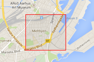
 To the right are two examples. The left image is quad
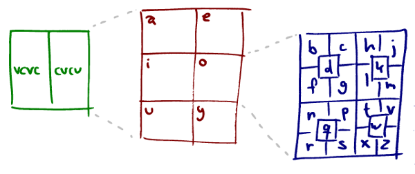
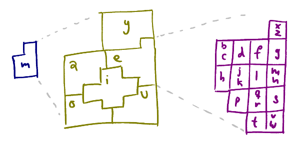
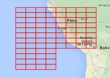

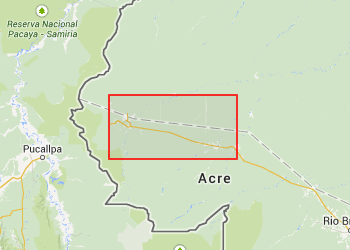

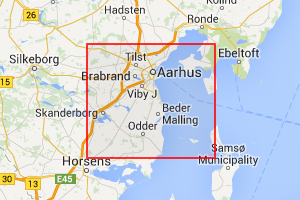
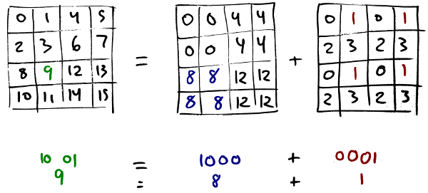
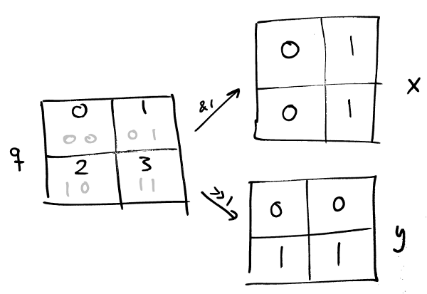
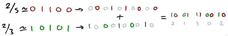
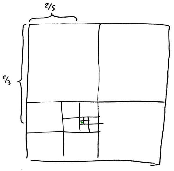
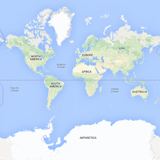
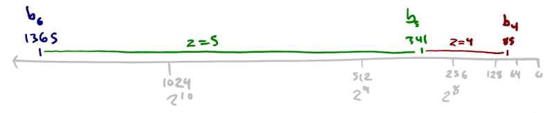
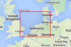
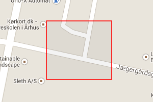
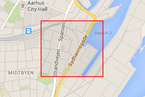

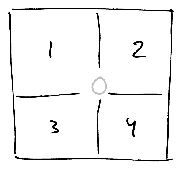

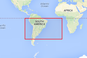

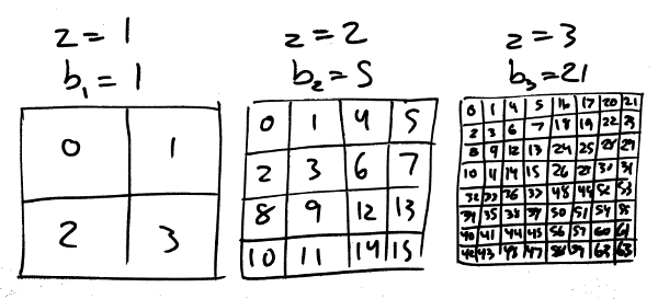
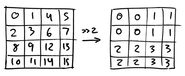
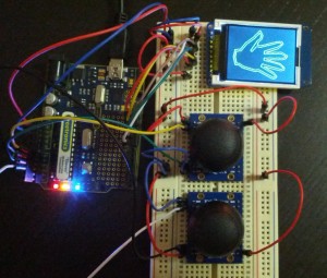

") ,
, ") , and so on, the Bezier defined by them is given by these parametric curves in x and y for t going between 0 and 1:
, and so on, the Bezier defined by them is given by these parametric curves in x and y for t going between 0 and 1: = x_0(1-t)^3 + 3x_1t(1-t)^2 + 3x_2t^2(1-t) + x_3t^3")
 = y_0(1-t)^3 + 3y_1t(1-t)^2 + 3y_2t^2(1-t) + y_3t^3")
") instead so I can write:
instead so I can write: = P_0(1-t)^3 + 3P_1t(1-t)^2 + 3P_2t^2(1-t) + P_3t^3")
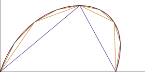 Using this definition you can draw a decent approximation of any Bezier curve just by plugging in values of t and drawing straight lines between the points you get out. The smoother you want the curve to be the more line segments you can use. On the right here is an example of using 2, 4, 8, 16, and 32 straight line segments. And on a small LCD you don’t need that many to get a decent-looking result.
 = K_0 + K_1t + K_2t^2 + K_3t^3")

")
")


 . Then the first four values we need for the differences are:
 = K_0")
=K_0+K_1d+K_2d^2+K_3d^3")
=K_0+2K_1d+4K_2d^2+8K_3d^3")
=K_0+3K_1d+9K_2d^2+27K_3d^3")


") from a
from a ") by doing:
by doing:


 is the same as
  except that the constant factor is left out. So


 we get
-1}=\frac{x}{\frac{x}{1!}+\frac{x^2}{2!}+\frac{x^3}{3!}+\cdots}=\frac{1}{\frac{1}{1!}+\frac{x}{2!}+\frac{x^2}{3!}+\cdots}")

\left(\frac{1}{1!} + \frac{x}{2!} + \frac{x^2}{3!} + \cdots\right)")

")
 + \frac{1}{1!}\left(\frac{1}{1!}B_1\right)")
+\frac{1}{2!}\left(\frac{1}{1!}B_1\right)+\frac{1}{1!}\left(\frac{1}{2!}B_2\right)")
!}\left(\frac{1}{0!}B_0\right)+\frac{1}{k!}\left(\frac{1}{1!}B_1\right)+\cdots+\frac{1}{1!}\left(\frac{1}{k!}B_k\right)")
=\frac{1}{k!}B_k")
!}\left(\frac{1}{0!}B_0\right)+\frac{1}{k!}\left(\frac{1}{1!}B_1\right)+\cdots+\frac{1}{k!}B_k")
!}\left(\frac{1}{0!}B_0\right)-\frac{1}{k!}\left(\frac{1}{1!}B_1\right)-\cdots-\frac{1}{2!}\left(\frac{1}{(k-1)!}B_{k-1}\right)")
!}\left(\frac{1}{0!}B_0\right)-\frac{k!}{k!}\left(\frac{1}{1!}B_1\right)-\cdots-\frac{k!}{2!}\left(\frac{1}{(k-1)!}B_{k-1}\right)")
!}\left(\frac{1}{0!}B_0\right)-\frac{k!}{k!}\left(\frac{1}{1!}B_1\right)=-\frac{1}{k+1}B_0-B_1=-\frac{1}{k+1}+\frac 12=\frac 12\cdot\frac{k-1}{k+1}")
!}\left(\frac{1}{2!}B_2\right)-\frac{k!}{(k-2)!}\left(\frac{1}{3!}B_3\right)-\cdots-\frac{k!}{2!}\left(\frac{1}{(k-1)!}B_{k-1}\right)")
!}\left(\frac{1}{2!}B_2\right)-\frac{k!}{(k-3)!}\left(\frac{1}{4!}B_4\right)-\frac{k!}{(k-5)!}\left(\frac{1}{6!}B_6\right)-\cdots")
!}B_2-\frac{k!}{4!(k-3)!}B_4-\frac{k!}{6!(k-5)!}B_6-\cdots")
!}B_2-\frac{2n!}{4!(2n-3)!}B_4-\frac{2n!}{6!(2n-5)!}B_6-\cdots")
!}B_1-\frac{2n!}{4!(2n-3)!}B_3-\frac{2n!}{6!(2n-5)!}B_5-\cdots")
 . So the above is the same as

+1)!} \quad \mathbf{for}\quad i > 0")
 \cdot 2n}{(1 \cdot 2 \cdots (2i-1) \cdot 2i)(2(n-i)+1)!}=\frac{(2n-(i-1))\cdot(2n-(i-2))\cdots (2n-1) \cdot 2n}{1 \cdot 2 \cdots i \cdot (i+1)}=\frac {2n}{2} \cdot \frac{2n-1}{3} \cdot\cdots\cdot \frac{2n-(i-1)}{i+1}")

")
")


}{i+1}\right)")

 , then
  , etc. We’ll the multiply those factors onto the previous Bi, which we’ve already been given, and accumulate the result in another variable,
  we’ll calculate directly:
 , and subtract it from the result:
 , we follow exactly the same pattern except that the factor is slightly different:
 :
:
 . But this is only an issue if you consider the program to calculate the whole Bernoulli sequence rather than just B7.