More Than Voronoi
This post is about a generalization of Voronoi diagram that I played around with. It’s probably not that useful but it’s a little fun math with an absolute ton of colorful diagrams.
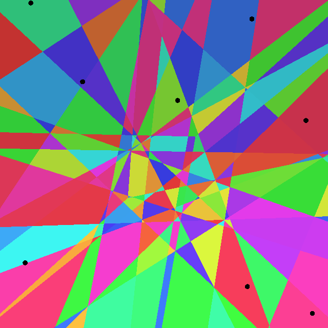
It occurred to me a while ago that there was a generalization of Voronoi diagrams that maybe could be useful to something I was working on. As you know, a Voronoi diagram divides the plane into regions based on a set of points. Given the points, p0, p1, …, pn, the region corresponding to pi is the set of points that are closer to pi than any of the other pj. Here is an example of a run-of-the mill, standard, plain vanilla, Voronoi diagram:

This diagram determines which points are closer using normal, cartesian, distance but Voronoi diagrams also make sense for other kinds of distance, for instance Manhattan distance:

The generalization that occurred to me was: if a region in a plain Voronoi diagram is defined by the one point it is closest to, what if you defined a diagram where regions are based on the two closest points? That is, for each pair of points, pi and pj, there would be a region made up of points where the closest point is pi and the second-closest is pj. What would that look like, I wondered. I searched around and it’s definitely a thing, it’s called a higher-order Voronoi diagram, but I couldn’t find any actual diagrams.
There may be some established terminology around this but I ended up using my own names: I would call what I just described a Voronoi2 diagram, and a plain one would be a Voronoi1. (From here on I’ll call the region around pi in the Voronoi1 diagram V(pi), and the region around pi and pj in the Voronoi2 diagram I’ll call V(pi, pj)).
You can kind of guess just from the definition that a Voronoi2 would look similar to the corresponding Voronoi1 just more subdivided. For any given pi, the point’s region in the Voronoi1 diagram, V(pi), is the set of point closest to pi. Well for any point in that set they will have some other point pj as their second-closest, and so if you take the union over all pj of V(pi, pj) that gives you V(pi). So the regions in a Voronoi2 diagram are basically fragments of regions of the Voronoi1.
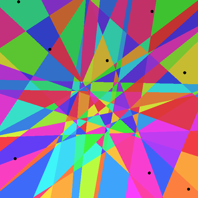
Below is the same diagram as before, for comparison, and the Voronoi2 diagram.


As you can see, that is exactly what the Voronoi2 diagram looks like: each Voronoi1 region has been subdivided into sub-regions, one for each of its neighboring points. You can do the same thing for the Manhattan diagrams,


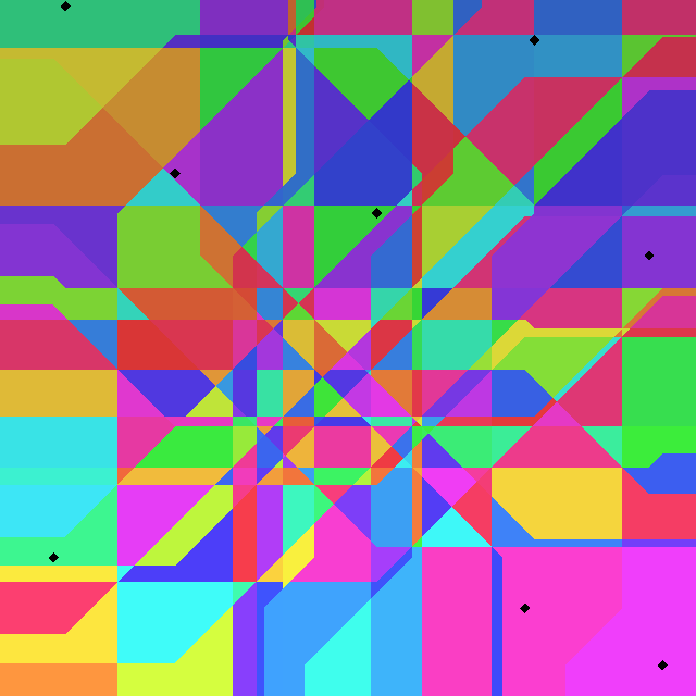
Now we’ve defined Voronoi1 and Voronoi2 but why stop there when we could keep going and define Voronoi3. This would be, you’ve probably already guessed it, a diagram with a region for each choice of pi, pj, and pk, that is made up of the points that have pi as their closest point, pj as their second-closest, and pk as their third-closest. Let’s call such a region V(pi, pj, pk). As I’m sure you’ve already guessed the Voronoi3 regions are further subdivisions of the Voronoi2 regions:


And the Manhattan version,


The images are becoming smaller but you can click them to see larger versions.
From here you can just keep going: Voronoi4, Voronoi5, Voronoi6, and so on and so on. Which of course I did, what did you expect? Here are Voronoi1-Voronoi8 with cartesian distance,


and the same with Manhattan distance


Except… I lied before when I said you could just keep going. In this example there are 8 points so the Voronoin diagrams are only well-defined for n up to 8 – that’s why there’s 8 diagrams above. And indeed if you look closely diagram 7 and 8 are actually the same – because once you’ve picked 7 points there is no choice for the last point, there is only the 8th left, so the diagrams end up looking exactly the same.
So is that it – is that all the colorful diagrams we get? Well, there is just one last tweak we can make to get a different kind of diagram.
The thing is, in the definition of Voronoi2 we said that V(pi, pj) was the points where pi is the closest point and pj is the second-closest. That is, the order of pi and pj is significant. An alternative definition we could use would be one where we don’t consider the order, where the region doesn’t care whether it’s pi closest and pj second-closest, or pj closest and pi second-closest. I’ll call this Vu(pi, pj) (the u is for unordered).
You’ll notice right away that by this definition Vu(pi, pj)=Vu(pj, pi) so there’s a lot fewer regions. Here’s an example of a Voronoiu1 (which is the same as the Voronoi1) and Voronoiu2 diagram,


With these unordered diagrams it can be a little trickier to figure out which two points a region actually corresponds to, especially in cases where the points in question are far away from the region. The trick you can use in this case is that for a given region is in the Voronoiu2, if you look at the same place in the Voronoi1 there will be a dividing line that goes across where the region is in the Voronoiu2, from one corner of the region to another. The two points on either side of the Voronoi1 will be the one the region corresponds to.
The same things works, as always, with Manhattan distance:


An interesting thing happens if we plot all the Voronoiun all the way up to 8:


The number of regions stays about the same and when we get to Voronoiu7 and Voronoiu8 they actually become simpler. This is because at that point the set of points for a given region includes almost all the points so the determining factor becomes which are the few points that aren’t in the set – and at 7 and 8 there’s 1 and 0 left respectively. So whereas Voronoi8 was useless because it’s the same as Voronoi7, here it’s useless because there’s only one region that contains all the points.
Is this construction at all useful? I’m not sure, I imagine it could be but I don’t have any particular use for them myself. Really I was just curious what it would look like.
I’ll leave you with a last set of diagrams, Voronoiu1 to Voronoiu8 for Manhattan distance.


