Category Archives: z-quads

This post is about giving a memorable name to every spot on the earth. It’s the fourth and probably last post in my series about z-quads, a spatial coordinate system. Previously I’ve written about their basic construction, how to determine which quads contain each other, and how to convert to and from geographic positions. This post describes a scheme for converting a quad to a memorable name and back again.

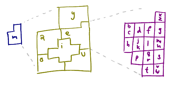
To the right are two examples. The left image is quad 10202 whose name is naga. The second is quad 167159511 whose name is naga hafy. As you might expect, naga hafy is contained within naga.

I can understand if at this point you’re thinking: what could possibly be the point of giving a nonsense name to every square on the surface of the earth?

What it’s really about is hacking your brain a little bit, encoding data using a pattern the brain is good at remembering instead of raw numbers which it isn’t. My original motivation was Ukendt Aarhus who takes pictures at inaccessible places in Århus and posts them on facebook, along with the position they were taken. I saw some of the pictures in real life and had to type a position like this

56.154382 / 10.20489

into google maps on my phone. My brain has absolutely no capacity for remembering numbers, even for a short while, so I have to do it a few digits at a time, looking back and forth. I’m much better at remembering words, even nonsense words. That is, I can hold more of this,

naga hazo yhes

in my head at once. Not the whole thing but certainly one word at a time, sometimes two. That’s the effect this naming scheme aims to use. Three words gives you a fairly precise location (a ~10m square) and if you need less, say to identify the location of a city, two words (a ~1km square) is typically enough. The town I grew up in, which is very small indeed, is uniquely identified by naga opuc.

Salad words

How do you generate reasonably memorable names automatically? The trick I used here is the one I usually use: alternate between consonants and vowels. It doesn’t always work but is usually good enough. I call those salad words (because “salad” is one).

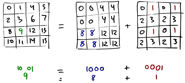
If you use just the English alphabet you have 6 vowels and 20 consonants. You can make 28800 four-letter salad words with those: two vowels (6²) times two consonants (20²) times 2 for whether the word starts with a consonant or a vowel. There are 21845 quads on the first 7 zoom levels so that will fit in one four-letter salad word.

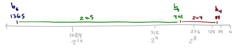
The first step in generating the string representation of a quad, then, is to split it into chunks that each hold 7 zoom levels. So if you want to convert quad 171171338190 which is at zoom level 19 you divide it into two chunks at level 7 and one chunk at level 5

10202   9941   974

This can be done using the ancestor/descendency operations from earlier. You can then convert each chunk into a word separately.

Encoding a chunk

There are many ways you could mape a value between 0 and 21845 to a salad word but one property I’d like the result to have is that it should give some hint about which area it covers, very roughly at least. I ended up with the following decomposition, (and let’s use zagi as an example while I describe how it works).

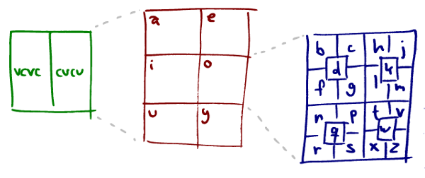
The world is divided into two parts along the Greenwich meridian. To the west words are vowel-consonant-vowel-consonant, to the east they’re consonant-vowel-consonant-vowel. So zagi must be east of Greenwich.

Each half is divided into six roughly evenly sized parts which determines what the first vowel is. (Note: not the first letter, the first vowel, which can be either the first or second letter.) The first vowel in zagi is a so it must be in the northwestern part of the eastern hemisphere. Each of the six divisions are subdivided 20 ways which determines the first consonant. The first consonant in zagi is z which is way down in the bottom right corner. This puts the location almost exactly in the middle of the eastern hemisphere. In fact, zagi is the quad that covers New Delhi.

The last two letters are determined in a similar way, further subdividing the region:

The second vowel determines a further subdivision, the second consonant narrows the quad down fully.

Now, the point of this is not for it to be possible to look at the name of a quad and know where it is – though the word ordering and first vowel rule sticks in your head pretty easily. The property it does have though is that at every level you have similar words grouped together geographically. These four maps show all level-7 quads that start with o, then on, then one, then finally onel.

      

      

If you know where onel is then you can be sure that onem is somewhere nearby.

The basic scheme is an attempt to exploit that we’re better at remembering word-like data than raw numbers. The subdivision scheme is a way to take that further and put some more patterns into the data. The brain is great at recognizing patterns.

In my experience it serves its purpose well: if you’re working within a particular area you become somewhat familiar with the quads by name and it becomes easier to remember things about them. One example is that coincidentally, Arizona is covered by quads starting with az, which is easy to remember. That gives you an anchor that helps you locate other a-quads because all the second consonants are located in a predictable way relative to each other. If you know where one is, that gives you a sense of where the others are.

I didn’t plan for that particular rule to be possible, I just noticed that I had started using it. And that’s the point: the patterns aren’t intended to be used or recognized in any particular way that I’ve anticipated in advance. They’re just available, like the grid on graph paper. How you actually remember them, or if you do at all, only emerges when you use the system in practice.

Implementation

The actual encoding/decoding is pretty straightforward but it’s tedious so I won’t go through it in detail, it’s in the source (js/java) if you’re curious. The shapes of the irregular subdivisions are encoded as a couple of tables.

The one bit that isn’t straightforward is the scheme for encoding the zoom levels 0-6. Remember, we’re not just encoding one zoom level but 8 of them. The trick when encoding a quad at the higher levels, 0-6, is to take the quad’s midpoint and zoom it down to level 7, keeping a bit saying whether we zoomed or not. Then encode the first three letters as if it were a level 7 quad initially and finally use the zoomed/not-zoomed bit to determine the last consonant. This is why there are two consonants in some of the cells in the purple diagram for the last consonant above. This works because if you take the midpoint of a quad levels 0-z and find cell at level z+1 that contains it, no other midpoint from 0-z will land in that same cell. So it’s enough to know whether we zoomed or not, if we did then there is a unique ancestor which must be the one we zoomed from.

Four-letter words

Another wrinkle on this scheme is that some four-letter salad words are, well, rude. Words you’d probably rather avoid if you have the choice. Since we’re only using 21845 of the 28800 possible words it’s easy to find an unused word near any one you’d like to avoid and manually map, for instance, 6160 to anux rather than anus.

There are many four-letter salad words left with meaning, even if you remove the rude ones. Like tuba, epic, hobo, and pony. Only 70% of words correspond to a valid quad so 30% of the meaningful words will not be valid. Of the ones that do a lot of them of them will be somewhere uninteresting like the ocean or Antarctica. But some do cover interesting places: pony and sofa are in WA, Australia, atom is near Vancouver, toga is in Papua New Guinea.

The toy site I mentioned in the last post also allows you to play around with quad names. Here is pony tuba,

The URL is,

http://zquad.p5r.org?name=pony-tuba

Further exploration

There’s a lot more you can do with z-quads, both as mathematical objects and as data structures.

On the data structure side spatial data structures and quad trees are well understood and it’s unclear how much new, if anything, you can do with z-quads. In my experience though they’re a convenient handle to use to describe and address data within spatial data structures.

As mathematical objects they have some nice properties and if you want to prove properties about them – for instance that a quad can contain at most one midpoint of a higher-level quad – they’re friendly to induction proofs. You can also easily generalize them, for instance to any number of coordinates. If you want to represent regular cubes instead of squares all the same tools work, they just have to be tweaked a bit:

b³_z = 1 + 8 + … + 8^z-1 + 8^z

ancestor³(q, n) = (q – b³_z) / 8ⁿ

The other way works too, with one dimension instead of two. That model gives you regular divisions of the unit interval.

This will probably be my last post about them though. It’s time to get back to coding with them, rather than writing about them.

This is the second post about z-quads, a spatial coordinate system. In the first post I outlined how they work and described how to jump between quads at different zoom levels. In this post I’ll look at how to determine whether one quad contains another, and how to find the common ancestor of two quads.

Containment

Given two quads q and s, how do we determine if q contains s? It’s pretty simple – there’s two cases to consider.

The one case is that the zoom level of q is higher than the zoom level of s. (Let’s call them z_q and z_s). If q is zoomed in more than s then it can’t contain s because it’s clearly smaller. So now let’s assume that q is at the same level or higher than s. If s is contained in q then that’s just another way of saying that q is s‘s ancestor. So if you get the ancestor of s that’s at the same level as q then you should get – q. In other words,

contains?(q, s) = (z_q ≤ z_s) and (ancestor(s, z_s – z_q) = q)

Pretty simple right? By the way, now you’re seeing why I pointed out before that the ancestor operation is defined for n=0: that’s what you’re using if you do contains?(q, q), which obviously you’d expect to be true.

This is the first operation where the zoom level appears explicitly and I’ll get into how to determine that for a given quad in a second. But first I’ll complete containment and talk about finding the most specific common ancestor of two quads.

Common ancestor

Let’s say we have two quads, call them q and s again, and you want to find the most specific ancestor of the two. That is, the ancestor that contains both of them and where no child also contain them both – since that would make the child more specific. This is well-defined since any two quads have, if no other, at least the trivial ancestor 0 in common.

The first step is to normalize q and s to the same zoom level. We’ll assume that s is zoomed in at least as much as q – if it’s not you can always just have an initial step that swaps them around. We can zoom s out to z_q and it won’t change what their common ancestor is because we know that is has to be at level z_q or above for it to be an ancestor of q. Let’s use t to refer to the result of zooming s out to q‘s level. So now we have q and t which are both a zoom level z_q.

To do the rest of the computation we need a bit more intuition about how the space of quad scalars is structured. As I’ve mentioned a few times at this point, because quads are numbered in z-order within one level all the descendants of a particular quad are contiguous, and so are the scalars. That means that you can split the binary representation of a scalar into 2-bit groups where each group corresponds to a subdivision of the whole space.

Here’s an illustration of how that works out for the scalars at zoom-2. You can think of the binary representation of the scalar, here for instance 9, as consisting of two groups: the top two bits indicate which 2×2 subdivision the quad belongs to, and the bottom two bits as the 1×1 subsubdivision within that one.

If you’re given two scalars, let’s take 9 and 11, and you write their binary representations together, then their common ancestor almost jumps out at you,

 9: 10 01
11: 10 11

You can tell from the top two bits that they’re both in the same subdivision but then they’re in different subsubdivisions. So the most specific common ancestor is the one that’s filled with 8s above.

This gives you a hint of how to find the most specific common ancestor more generally: you take the two scalars, then you see which 2-bit groups are different, and then you zoom out just enough that you discard all the groups that are different and keep the ones that are the same. You can find the highest bit where two numbers are different by xor’ing them together and taking the highest 1-bit in the result:

   9: 10 01
  11: 10 11
 xor: 00 10

Here the highest different bit is at 2 so they’re different at the lowest zoom level but then they’re the same. So their most specific common ancestor is the quad you get by zooming out one step from either of them. More generally, the formula for getting the most specific common ancestor of two quads q and t at the same zoom level z is,

msca(q, t, z) = ancestor(q, ffs((q – b_z xor t – b_z) + 1) / 2)

Here ffs is find-first-set which returns the index of the highest 1-bit in a word, 0 if there are none. The (x+1)/2 part is to get from a bit index to a zoom level. For instance if the highest set bit is 1 or 2, as in the example, (x+1)/2 will be 1.

At this point let’s just recap quickly. Given a quad you can get an ancestor, a descendant, and you can determine how it is related to any of its ancestors. Given two quads you can determine whether one contains the other, and you can find the most specific common ancestor. All in a constant, low, number of bit operations. There are more operations to come but already I think we’ve got a big enough library of operations to be useful.

I’ve glossed over a few things along the way though, particularly how to determine the zoom level for a given quad. That’s what I’ll talk about next. It’s kind of fiddly so if you’re okay with trusting that it can be calculated efficiently then you can just skip this part and go on to the part where I talk about how to convert from regular floating point coordinates to quads and back.

Otherwise, let’s go.

Zoom

Given a quad, what is its zoom level?

Since quads at higher zoom levels have higher numeric values one way to answer this is to just compare with the biases. If a value is between b₄ and b₅ then it must have zoom level 4, and so on. Since the biases are sorted you can even do binary search. But you can be a lot smarter than that.

Here’s an illustration of where the quads at zoom level 4 and 5 are located on the numbers line,

The zoom-4 quads start at 85 and end at 340, then the zoom-5 quads start at 341 and run until 1364 where zoom-6 starts. Each range of quads contains values from three different 2-power intervals: zoom-4 contains values from the 2⁶ to the 2⁸ interval, zoom-5 from 2⁸ to 2¹⁰, and so on. This suggests that determining the highest set one-bit in the quad is a good place to start.

As an example, say the highest one-bit is 8 or 9. That is, the quad is between 256 and 1024. If you look at the numbers line then you see that there are two possibilities: if it’s smaller than b₅, 341, then it’s at level 4, otherwise it must be at level 5. Similarly, if the highest bit is at index 10 or 11, that is a value between 1024 and 4096, then the level is 5 or 6 depending on whether the quad is larger than b₆, 1365.

There’s a general principle working here. Say highest set bit of a quad is at index k. The zoom level will be c=k/2 if the quad is is smaller than b_c+1, otherwise it’s c+1.

As an illustration, let’s try this with one of the quads from the introduction, 171171340006. The highest 1-bit is at index 37 so c is 18. This means that that quad is at zoom level 18 or 19. The boundary between the two is b₁₉ which is 91625968981. This is less than the quad’s value so the result must be 19.

Okay so this almost gives us a fast way to calculate the zoom level. The one thing that’s missing is: how to get an arbitrary zoom bias quickly – how do you know that b₁₉ is 91625968981? There’s only a small number of bias values of course so you can just put them in a table, but you can also calculate them directly. The thing to notice is that the binary representation of a bias is simple:

b3: 10101 (= 21)     
b4: 1010101 (= 85)   
b5: 101010101 (= 341)

…and so on. They’re all alternating ones and zeroes. That’s because, as we saw before, they are made up of sums of powers of 4. That gives us a practical way to calculate them: take the binary number that consists of alternating 0s and 1s and mask out the bottom part of the appropriate size. So for b₃ we mask out the bottom 5 bits, for b₄ the bottom 7 and so on:

bz = 0x5555555555555555 & ((1 << 2 z) - 1)

I imagine there might be more efficient ways but this one works.

Calculating the zoom level isn’t particularly expensive but you need it for most operations so in my own code I typically compute it once early on and then keep it cached along with the quad itself (though it’s not something you would ever store or transmit along with the quad since it’s redundant). Even for some of the operations where you technically don’t need it it’s still useful to have it. For instance, you can get nth ancestor of a quad without knowing the zoom, but the operation is only well-defined if the quad’s zoom is n or greater so it’s nice to have the zoom around so you can make that assertion explicitly in the code.

I think that’s enough for one post. In the next part we’ll talk about how to do conversion between coordinates and quads.