Category Archives: babbage

Bernoulli

It’s Ada Lovelace‘s 197th birthday today and the perfect day for my last post about Babbage‘s computing engines. This one is about the famous first program for calculating the Bernoulli series which appeared in Note G of her notes on Babbage’s analytical engine. One of the odd things about this program is that it’s widely known and recognized as an important milestone – but as far as I can determine not widely understood. I haven’t found even one description of what it does and how it does it, except for the original note.

In this post I’ll give such a description. It has roughly three parts. First I’ll give a quick context – what is Note G, that kind of thing. Then I’ll derive the mathematical rules the program is based on. I’ll roughly follow the same path as Note G but I’ll include a lot more steps which should make it easier to digest. Note G is very concise and leaves a lot of steps to the reader and the derivation is quite clever so some of those steps can be tricky. (You can also just skip that part altogether and take the result at the end as given.)

In the last part I’ll write up a modern-style program in C that does the same as the Note G program and then break it down to get the program itself. Finally I’ll do what you might call a code review of the program.

Okay, let’s get started.

Background

I won’t go into too many general details about Babbage, Ada Lovelace, or the analytical engine. There’s plenty of resources on them and their history on the web, including other posts I’ve written about the difference engine (what motivated ithow did it work) and programming the analytical engine (table code, microcode, and punched cards).

In 1840, after Babbage had been working on the analytical engine for a while, he went to Turin and discussed his ideas with a group of engineers and mathematicians. Based on those conversations one of them, Luigi Menabrea, published an article about the engine in French in 1842. Soon after that Ada Lovelace translated the article into English and Babbage encouraged her to write an original article. She did – sort of – but rather than write a separate article she did it in the form of notes to her translation of Menabrea’s article. Just to give an idea of how much she added, her translation with notes, published in 1843, was three times as long as the original. One of the notes, Note G (they were named from A to G), presented the program I’ll describe in this post.

We’ll get to that very soon but first a few words about what it calculates, the Bernoulli series.

Bernoulli

This is the first few values of the Bernoulli series:

Name B0 B1 B2 B3 B4 B5 B6 B7
Value 1 -1/2 1/6 0 -1/30 0 1/42 0

It’s one of those mathematical objects, like e and π, that keep appearing in different places and seem to have a special significance within the structure of mathematics. One place it appears is in Taylor expansions of exponential and trigonometric functions – for instance, it holds that

  \frac{x}{e^x-1} = \sum_{i=0}^{\infty}\frac{x^i}{i!}B_i = \frac{1}{0!}B_0 + \frac{x}{1!}B_1 + \frac{x^2}{2!}B_2 + \cdots

The Bernoulli series is not that difficult to compute but it’s not trivial either. If you want to demonstrate the power of a computing engine it’s not a bad choice.

Part of Note G is concerned with deriving a way to calculate the series and that’s what we’ll start with, using the formula above in combination with a second identity, one you’re probably already familiar with, the Taylor expansion of ex:

  e^x = \sum_{i=0}^{\infty}\frac{x^i}{i!} = \frac{1}{0!} + \frac{x}{1!} + \frac{x^2}{2!} + \cdots

If we plug this into the left-hand side of the previous equation in place of e^x we get

  \frac{x}{e^x-1} = \frac{x}{\left(\frac{1}{0!} + \frac{x}{1!}+\frac{x^2}{2!}+\cdots\right)-1}=\frac{x}{\frac{x}{1!}+\frac{x^2}{2!}+\frac{x^3}{3!}+\cdots}=\frac{1}{\frac{1}{1!}+\frac{x}{2!}+\frac{x^2}{3!}+\cdots}

This means that the original equation can also be written as

  \frac{1}{\frac{1}{1!} + \frac{x}{2!} + \frac{x^2}{3!} + \cdots} =\frac{1}{0!}B_0+\frac{x}{1!}B_1+\frac{x^2}{2!}B_2+\cdots

Multiplying the denominator from the left-hand side onto both sides we get this identity:

  1 = \left(\frac{1}{0!}B_0+\frac{x}{1!}B_1+\frac{x^2}{2!}B_2+\cdots\right)\left(\frac{1}{1!} + \frac{x}{2!} + \frac{x^2}{3!} + \cdots\right)

This looks like we’ve gone from bad to worse, right? Both series on the right are infinite and we have an inconvenient variable x stuck in there which we need to get rid of. This is where the cleverness comes in.

We’re not going to multiply these two series together, but if we were to do it we know what the result would look like. It would be a new series in x of the form:

  c_0+c_1x+c_2x^2+\cdots

The 1 on the left-hand side even tells us what those coefficients are going to be: c0 is going to be 1 and all the remaining cis are going to be 0. And even though the full product will be infinite, the individual coefficients are all nice and finite; those we can derive. Here is the first one, which we know will be 1:

  1 = c_0 = \frac{1}{1!}\left(\frac{1}{0!}B_0\right)

The only unknown here is B0 and if we solve for it we get that it’s 1. Let’s try the next one:

  0 = c_1 = \frac{1}{2!}\left(\frac{1}{0!}B_0\right) + \frac{1}{1!}\left(\frac{1}{1!}B_1\right)

Since we now know what B0 is B1 is the only unknown; solving for it gives us -1/2. One more time,

  0 = c_2 = \frac{1}{3!}\left(\frac{1}{0!}B_0\right)+\frac{1}{2!}\left(\frac{1}{1!}B_1\right)+\frac{1}{1!}\left(\frac{1}{2!}B_2\right)

Solving for B2 gives us 1/6.

In general, if we know the first k-1 Bernoulli numbers we can now calculate the k‘th by solving this:

  0 = c_k = \frac{1}{(k+1)!}\left(\frac{1}{0!}B_0\right)+\frac{1}{k!}\left(\frac{1}{1!}B_1\right)+\cdots+\frac{1}{1!}\left(\frac{1}{k!}B_k\right)

This only gets us part of the way though, it needs to be cleaned and simplified before we can code it. (And again, if you find yourself getting bored feel free to skip to the next section where we start coding).

The first simplification is to solve Bk up front. As you can see above the term we’re interested in is always the last one and has the form

\frac{1}{1!}\left(\frac{1}{k!}B_k\right)=\frac{1}{k!}B_k

This we can solve for in the original equation:

  0 = \frac{1}{(k+1)!}\left(\frac{1}{0!}B_0\right)+\frac{1}{k!}\left(\frac{1}{1!}B_1\right)+\cdots+\frac{1}{k!}B_k

  \frac{1}{k!}B_k=-\frac{1}{(k+1)!}\left(\frac{1}{0!}B_0\right)-\frac{1}{k!}\left(\frac{1}{1!}B_1\right)-\cdots-\frac{1}{2!}\left(\frac{1}{(k-1)!}B_{k-1}\right)

  B_k=-\frac{k!}{(k+1)!}\left(\frac{1}{0!}B_0\right)-\frac{k!}{k!}\left(\frac{1}{1!}B_1\right)-\cdots-\frac{k!}{2!}\left(\frac{1}{(k-1)!}B_{k-1}\right)

This simplifies the process of calculating Bk, we now just have to plug the previous values into this equation to get the next one.

We’ve already computed the first few values of the series so we can calculate the first two terms up front:

  -\frac{k!}{(k+1)!}\left(\frac{1}{0!}B_0\right)-\frac{k!}{k!}\left(\frac{1}{1!}B_1\right)=-\frac{1}{k+1}B_0-B_1=-\frac{1}{k+1}+\frac 12=\frac 12\cdot\frac{k-1}{k+1}

Pluggin them back into the formula we get:

  B_k=\frac 12\cdot\frac{k-1}{k+1}-\frac{k!}{(k-1)!}\left(\frac{1}{2!}B_2\right)-\frac{k!}{(k-2)!}\left(\frac{1}{3!}B_3\right)-\cdots-\frac{k!}{2!}\left(\frac{1}{(k-1)!}B_{k-1}\right)

As the table of Bernoulli values at the beginning suggested all the numbers at odd indexes greater than 1, B3B5, etc., are zero. And since we’ve already handled 1 as a special case we can just drop all the odd terms:

  B_k=\frac 12\cdot\frac{k-1}{k+1}-\frac{k!}{(k-1)!}\left(\frac{1}{2!}B_2\right)-\frac{k!}{(k-3)!}\left(\frac{1}{4!}B_4\right)-\frac{k!}{(k-5)!}\left(\frac{1}{6!}B_6\right)-\cdots

Above each Bi has two separate factors being multiplied onto it; we can multiply those together to make just one factor:

  B_k=\frac 12\cdot\frac{k-1}{k+1}-\frac{k!}{2!(k-1)!}B_2-\frac{k!}{4!(k-3)!}B_4-\frac{k!}{6!(k-5)!}B_6-\cdots

Since we’re only even interested in even values of k we don’t lose generality if we assume that that k=2n for some integer n.

  B_{2n}=\frac 12\cdot\frac{2n-1}{2n+1}-\frac{2n!}{2!(2n-1)!}B_2-\frac{2n!}{4!(2n-3)!}B_4-\frac{2n!}{6!(2n-5)!}B_6-\cdots

Okay, now we’re getting close to the final form that we’ll code up but first I’ll have to stop and do something distasteful: I’ll change how we denote the values in the Bernoulli series. What you’ve seen up until this point is the modern, standard use of indices: B1 is -1/2, B2 is 1/6, B3 is 0 etc. In Note G, however, Lovelace numbers the values differently. She skips the first two values and the rest are shifted by 1 so that B1 denotes the value we would call B2, B2 is what we would call B3 and so on:

Value 1 -1/2 1/6 0 -1/30 0 1/42 0
Modern B0 B1 B2 B3 B4 B5 B6 B7
Note G not used B1 B2 B3 B4 B5 B6

Up until now I’ve been using (what we call) B0 and B1 so it made sense to use the modern convention but now we only have terms left that have a name in Note G, so I’ll switch to her convention. This means that I’ll write the formula as

  B_{2n-1}=\frac 12\cdot\frac{2n-1}{2n+1}-\frac{2n!}{2!(2n-1)!}B_1-\frac{2n!}{4!(2n-3)!}B_3-\frac{2n!}{6!(2n-5)!}B_5-\cdots

Note that the meaning of n doesn’t change so the formula is almost the same as it was before, the only difference is the numbering of the Bis.

At this point it’s convenient to give the factors being multiplied onto Bi a name; we’ll call them A^n_i. So the above is the same as

  B_{2n-1}=A^n_0-A^n_1B_1-A^n_3B_3-A^n_5B_5-\cdots-A^n_{2n-3}B_{2n-3}

where

A^n_0 = \frac 12\cdot\frac{2n-1}{2n+1}

A^n_i = \frac{2n!}{2i!(2(n-i)+1)!} \quad \mathbf{for}\quad i > 0

The second one looks hairy but can be boiled down:

  \frac{1 \cdot 2 \cdots (2n-1) \cdot 2n}{(1 \cdot 2 \cdots (2i-1) \cdot 2i)(2(n-i)+1)!}=\frac{(2n-(i-1))\cdot(2n-(i-2))\cdots (2n-1) \cdot 2n}{1 \cdot 2 \cdots i \cdot (i+1)}=\frac {2n}{2} \cdot \frac{2n-1}{3} \cdot\cdots\cdot \frac{2n-(i-1)}{i+1}

The last step is possible because there is, very conveniently, the same number of terms in the numerator and denominator. What’s useful about this form is that it makes it clear that each of the Ais is the previous one with another factor multiplied onto it (except for A0 which is special):

  A^n_1 = \frac{2n}{2}

  A^n_2=\frac{2n}{2}\cdot\frac{2n-1}{3}=A^n_1\left(\frac{2n-1}{3}\right)

  A^n_3=\frac{2n}{2}\cdot\frac{2n-1}{3}\cdot\frac{2n-2}{4}=A^n_2\left(\frac{2n-2}{4}\right)

We’re slowly starting to see a program take shape here: if we know the previous Bi we can iteratively calculate the sequence of Ais and multiply them onto those values, ultimately giving us the next Bi. Now we’ll switch gears and code that up as an actual program.

The program

Let’s quickly recap what all the work above gave us. This formula gives us the next Bernoulli number, given the previous values:

  B_{2n-1}=A^n_0-A^n_1B_1-A^n_3B_3-A^n_5B_5-\cdots-A^n_{2n-3}B_{2n-3}

where

  A^n_0=\frac 12 \cdot \frac{2n-1}{2n+1}

  A^n_1=\frac {2n}{n}

  A^n_i=A^n_{i-1}\left(\frac{2n-(i-1)}{i+1}\right)

Say we wanted to write a program that calculated B7 using this approach, that is, the special case where n is 4 (since, as you may vaguely remember, n is the value such that k = 2n – 1).

  B_7=A^4_0-A^4_1B_1-A^4_3B_3-A^4_5B_5

Let’s take a crack at implementing this in C. We’ll do it twice: first a straightforward implementation that’s quite similar to the Note G program and then we’ll go back over it again and make some modifications to make is (almost) step-by-step identical to Note G.

First, we can assume that the program has been given n and that we have already computed the preceding Bi. We’ll store those in some variables.

double n = 4;
double B1 = 0.166667;                             // 1/6
double B3 = -0.0333333;                           // -1/30
double B5 = 0.0238095;                            // 1/42

The general idea will be to keep a variable A that we’ll multiply successive factors onto so it takes the value of A^4_1, then A^4_3, etc. We’ll the multiply those factors onto the previous Bi, which we’ve already been given, and accumulate the result in another variable, result.

The first term A^4_0 we’ll calculate directly:

double A = 0.5 * (2 * n - 1) / (2 * n + 1);       // A0
double result = A;

Then we calculate the second term, A^4_1B_1, and subtract it from the result:

A = 2 * n / 2;                                    // A1
double term = B1 * A;                             // B1 A1
result -= term;                                    // A0 - B1 A1

The we calculate A^4_3 by multiplying the appropriate factor onto A^4_1:

A *= (2 * n - 1) / 3 * (2 * n - 2) / 4;           // A3
term = B3 * A;                                    // B3 A3
result -= term;                                   // A0 - B1 A1 - B3 A3

And for the last term, A^4_5B_5, we follow exactly the same pattern except that the factor is slightly different:

A *= (2 * n - 3) / 5 * (2 * n - 4) / 6;           // A5
term = B5 * A;                                    // B5 A5
result -= term;                                   // A0 - B1 A1 - B3 A3 - B5 A5
printf("The result is: %g\n", result);

If you run this program it will print

The result is: -0.0333333

which is indeed –1/30 also known as B7. This is, in essence, what the Note G program does. It calculates B7 using this sequence of steps. However, if you were to look at Note G now what you’d see would still look a bit foreign. That’s because C let’s us do things that the analytical engine doesn’t. For instance, C lets us write complex expressions where the analytical engine only does one operation at a time. In C we also don’t need to worry about recurring expressions like n * 2 because the compiler will make sure it only gets calculated once. The analytical engine obviously had no compiler so the programmer has to do that kind of optimizations by hand.

To take all this into account I’ll rewind and go over the program again but this time I’ll include all the extra work. In the code comments I’ll give how the variables in my program maps to variables in Note G.

First off we have the values we’re given as input:

one = 1.0;                                        // V1
two = 2.0;                                        // V2
n = 4.0;                                          // V3
B1 = 0.166667;                                    // V21
B3 = -0.0333333;                                  // V22
B5 = 0.0238095;                                   // V23

Note G doesn’t use constant values, only variables. So to use the values 1 and 2 it needs two variables that are pre-initialized with those values. Also, we’ll assume that all variables are pre-declared and start out with the value 0, we won’t bother declaring then anymore.

The first step is to calculate A^4_0. The C version was:

double A = 0.5 * (2 * n - 1) / (2 * n + 1);       // A0
double result = A;

and here is the same thing in analytical-engine-style C:

two_n_minus_one = two_n_plus_one = numerator = two * n;  // V4 V5 V6
two_n_minus_one -= one;                           // V4
two_n_plus_one += one;                            // V5
A = two_n_minus_one / two_n_plus_one;             // V11
A /= two;
result += A;                                      // V13
current_n = n - one;                              // V10

If you compare the two versions it should be clear that they do the same thing except that in the latter you get all the excruciating details of the temporary variables. But it’s still pretty straightforward. Notice in the next to last step how we add A to result before result has ever been assigned – we’re using the fact that variables that haven’t been used yet can be assumed to be 0.

The next part of the C program calculates A^4_1B_1:

A = 2 * n / 2;
double term = B1 * A;                             // B1 A1
result -= term;                                    // A0 - B1 A1

In analytical-engine-style this corresponds to:

denominator += two;                               // V7
A = numerator / denominator;
term = B1 * A;                                    // V12
result -= term;
current_n -= one;

Instead of recalculating 2*n we already have it in a variable, numerator, and will be decrementing it as we go. Similarly with the denominator which we’ll increment as we go rather than recalculate. Notice again how we increment denominator before it has been initialized and rely on it being 0 so it ends up containing 2.

The next step is to calculate A^4_3B_3:

A *= (2 * n - 1) / 3 * (2 * n - 2) / 4;           // A3
term = B3 * A;                                    // B3 A3
result -= term;                                   // A0 - B1 A1 - B3 A3

In analytical engine style we get:

numerator -= one;
denominator += one;
factor_1 = numerator / denominator;               // V8
A *= factor_1;

numerator -= one;
denominator += one;
factor_2 = numerator / denominator;               // V9
A *= factor_2;

term = B3 * A;
result -= term;
current_n -= one;

The first two blocks together calculate A^4_3 and the last part subtracts another term from result. The last part looks very similar:

A *= (2 * n - 3) / 5 * (2 * n - 4) / 6;           // A5
term = B5 * A;                                    // B5 A5
result -= term;                                   // A0 - B1 A1 - B3 A3 - B5 A5

In this code we’re using different constants to calculate A than the previous block, and we’re using B5 instead of B3 in the second step. In the analytical-engine-style code we’ve already decremented the variables we’re using to calculate A so that part is exactly the same as for the previous block, but we still need to use B5 instead of B3:

numerator -= one;
denominator += one;
factor_1 = numerator / denominator;
A *= factor_1;

numerator -= one;
denominator += one;
factor_2 = numerator / denominator;
A *= factor_2;

term = B5 * A;
result += term;
current_n -= one;

That’s it – the value of B7 is now stored in result. The only thing left to do is to store the value in a dedicated variable and then reset some of the other variables so we’re ready to calculate the next Bi.

B7 += result;                                     // V24
n += one;
// Also reset numerator and denominator.

Now, it might look like we’ve just written the world’s most excruciating C program. In fact what’s we’ve done here is step through, instruction-by-instruction, the Bernoulli program in Note G. If you look through that program here on the right you will notice that for each step there is a corresponding line in the analytical-engine-style C program above. (For details on how the table program format works see my post on analytical programming.) Click the program to go to an expanded version.

Comparing the programs

Now, if you were to go though the program in details you would notice that what I just said isn’t actually true. There are some small differences between the C-style version and what you see in the original notes. Those differences are, I’m afraid, bugs in the original program.

There are three separate issues. The first one is trivial: in step 4 the instruction that should do

A = two_n_minus_one / two_n_plus_one;

is actually switched around and does

A = two_n_plus_one / two_n_minus_one;

That’s a tiny issue that could have been introduced by the printer, and the comment for that step in the table has it the right way round.

Secondly, remember how similar the code for calculating A^4_3B_3 and A^4_5B_5 was, the only difference being that one used B3 and the other B5? The second issue is that Note G actually overlooks this difference and where the code for A^4_5B_5 should be simply says to repeat the steps for calculating A^4_3B_3. As you’ll see if you click through to the expanded version, in the white space between steps 23 and 24 there is a comment saying “Here follows a repetition of Operations thirteen to twenty-three”.

The third issue is more systematic: the signs are reversed. If you fix the two first issues the result will be correct – except that it has the wrong sign. The sign reversal is also present in the text of the note so I’m not sure if it’s deliberate, but if it is the program calculates something we wouldn’t call the Bernoulli series.

There is also a fourth bonus issue, which is not a bug exactly. At the end in step 25 the code resets some variables such that it’s ready to calculate B9. But if you loop around and run the main program again it won’t give the right result. This is both because some of the variables which the program assumed were 0 on the first run won’t be on the second and because the “loop” after step 23 would need yet another block, this one for calculating A^5_7B_7. But this is only an issue if you consider the program to calculate the whole Bernoulli sequence rather than just B7.

Now, I want to be sure to put these issues in the right perspective. This is a complex program. I’ve been programming most of my life and it still took me a significant amount of time to understand how it worked. This program was written by a mathematician with no background in programming – they were inventing programming as they went along. On paper. There is an almost frightening intellectual power behind this, both in the program itself and the underlying framework. For me, the fact that we modern programmers, with the benefit of education and experience, can spot a few details out of place is only what you would expect and takes little away from that.

That’s it, you now know how the Note G program works and what each step does. If you’ve found this interesting there’s a good chance you’ll find Lovelace’s original notes interesting too, I recommend reading them. If you want to play around with the program yourself I’ve “ported” it to C; you can find it on github.

Punched Cards

This post is a continuation of analytical programming about the programming model used to program Babbage’s analytical engine. In the previous post I talked about two of the ways programming was used, the table format used to describe programs and the microcode format used internally within the engine. The third program format which is what this post is all about is the one used to feed programs to the engine. (Side note: if this looks familiar it’s because it used to be the second half of that post which you may already have read; I’ve just pulled it out into a separate post)

In some regards the card format is similar to the bytecode formats we know today. That’s one of the reasons I find it especially interesting, because it’s so relatively familiar and relatable for a modern programmer. However, in one regard is is very different from any modern programming model. Babbage felt very strongly that there was a fundamental difference between specifying which operation to perform and which variables to perform the operation on. Modern programming and mathematics has generally moved in the opposite direction, seeing operations and function as values of a different type that can nonetheless be abstracted over much the same way that numeric values can. Babbage would have disagreed strongly with this.

Because of this view a punched card program is divided into two distincts parts: one set of cards containing all the operations to perform and another set specifying the variables to perform them on. For instance, a program that multiplied three numbers, V1, V2, and V3 and stored the result in V4, similar the table program from the previous post but using multiplication instead of addition, would be split from the format where operations and variables are together,

V1 × V2 → V4
V3 × V4 → V4

and into two separate sets of cards, one giving the operations

×
×


and one giving the column indices

1
2
4
3
4
4


In the following I’ll use these colored boxes to represent punched cards. The real punched cards didn’t look anything like this as you’ve seen from the picture at the beginning. For the variable cards I’m also omitting the part that indicates whether reads are clearing or restoring, that would have been there in the original design.

Besides specifying which operation to perform the operation cards all specified how many times the operation should be repeated; using this the operations program above could be specified even more succinctly as

×
2


1
2
4
3
4
4


To execute an instruction the engine would first read the operations card and store the number of repeats in a register, the Operation Card Counting Apparatus. Then it would repeatedly perform the operation, decrementing the O.C.C.A for each and reading the next operation card when it reached zero. For each operation it would read as many variable cards as were appropriate for that operation.

In the following I’ll describe each of the instructions understood by the engine. It’s only about a dozen. The number of variable cards for an operation card depends on the repeat count but I’ll show the variable cards that go with a single repetition. I’ll separate the cards representing input and output with an arrow, just to make it easier to read. It’s purely a visual aid though, in practice you had to keep track what the cards meant yourself.

Basic Operations

The most straightforward arithmetic instructions, instruction format wise, are the multiplicative ones. We have multiplication of two columns, Vi and Vj:

×
n


Vi
Vj
Vh
Vm
Vt


Wait, you might say, didn’t you just show multiplication using just three variable cards? Yes, and that was a simplification. In reality multiplying two 50-digit numbers can give you up to 100 digits and as a general principle the analytical wouldn’t discard digits. Instead it would store the most significant 50 digits in one column and the least significant 50 in another. In addition, unlike the difference engine the analytical engine had built-in support for fixed-precision values by allowed you to specify an implicit multiplier which would be taken into account during all operations. This could cause a single multiplication to produce up to 150 digits, hence you need three columns to be able to store the result of any multiplication, called the head, middle, and tail values. If you know your output fits within 50 digits you can use scratch columns for the most significant parts and only use the least significant 50 bits of the output, that’s up to you, but you always have to pass three output variable cards.

Symmetric to multiplication the engine also supported division:

÷
n


Vi
Vj
Vh
Vm
Vt


The input/output logistics of this operation are the same as multiplication, the result can be up to 150 digits long. The microcode for division is even more complex than multiplication, as you would probably expect. It’s an iterative approach that first approximates the result by looking just at the most significant digits of both inputs and gradually refines the result by considering more and more less significant digits. Both operations take time proportional to the number of digits of the numbers involved.

Besides arithmetic operations the engine also supported shifting values up and down in base 10, corresponding to multiplying or dividing by powers of 10. Here is the step down operation, what we would call right-shifting:

>
n
#
a


Vi
Vh
Vt


This instruction shifts the value in Vi a steps to the right, effectively dividing the value by 10a. The n as usual specifies how many times to repeat the operation. Like with the multiplicative operations the shift, sorry stepping, operations are somewhat familiar but also quite different. The step up operation takes two parameters: the number of times to repeat the operation and how far to shift the value. Since each operation card only holds one parameter and this one uses two we need to operation cards, the operation itself and a dummy card that has no function but to hold the amount to shift by.

In modern programming shift operations always discard bits, either high or low bits. As we’ve seen Babbage made sure operations never discarded bits. In this case we get two outputs: the shifted value on one column and the bits that were shifted away on the other. Again, if you really intend to discard the bits that were shifted away you can just store them in a scratch column.

Internally the engine had primitives that could shift by 1 and 2 digits in one cycle and the shift card was implemented by repeatedly shifting by 1 digit. If you wanted to shift by an even number there was a separate card that worked the same way as the single shift but repeating the 2-digit shift primitive:

>>
n
#
a


Vi
Vh
Vt


This instruction shifts by 2a but uses only a cycles to do it where the single step down operation would take 2a cycles. Symmetrically there are operations for stepping up, what we would call shifting left:

<
n
#
a


Vi
Vh
Vt


<<
n
#
a


Vi
Vh
Vt


There’s a few things to note about this set of operations. First of all, the amount to shift by is always fixed by an operation card so there is no way to shift by a variable or computed amount, only by a constant. Also, since no values are ever discarded the up/down variants are complementary: stepping up by 26 gives you the same result as stepping down by 24 except that the head and tail of the results are swapped. So you would never step more than 25 in any direction because you could get the same result with fewer cycles by stepping the other way.

Now we get to addition and subtraction. You might think they were among the simpler operations, simpler than division surely, but no, the instruction format is really hairy. The thing is, you very often end up having to perform long sequences of additions and subtractions and if the format was straightforward like division you would end up constantly writing values out to columns and reading them back in. What you really want is to add and subtract a sequence of numbers into a running sum inside the engine’s mill and only once you’ve done store the result in a column. The interface for doing this changed many times and the final result is clearly a work in progress itself. The basic form looks like this:

+
a
b
+


Vi0
Vi1
Via
Vj0
Vj1
Vjb
Vo


This instruction first adds a values together, then subtracts b values, and finally stores the result in Vo. The second addition card seems a bit random; it’s not clear why it’s even necessary but in any case it’s just an end marker, it doesn’t cause any numbers to be added.

You might be thinking to yourself: surely you need two columns to store the result or you may end up discarding digits? Well yes, sort of. The internal column that stores the running total before it’s transferred out has 3 extra digits of precision so you can safely add and subtract lots of numbers without overflowing. And as long as you’re sure that the final result doesn’t exceed 50 digits then you’re good. If the result does exceed 50 digits then the machine would stop and notify the machine’s operator, presumably by ringing a bell. What he could do to resolve the issue is unclear. But that’s how it worked.

Now, Babbage felt that this was a somewhat limited interface: you have to add first, then subtract, and then you’re done. Sometimes you want to subtract first. Other times you want to add, then subtract, then add some more, and so on. So he experimented with other approaches, like allowing as many add and subtract cards as you want, in any order, terminated by a special F card. Often you want just one addition or subtraction so he introduced two new cards, add-once and subtract-once. Why that’s better than a general add card with a repetition count of one is unclear but presumably they were faster. This was still a work in progress and we don’t know how addition would ultimately have worked if he’d been able to complete his design.

Special operations

The operations I’ve covered so far are the most straightforward ones, the arithmetic operations. The remaining ones are a set of somewhat obscure arithmetic operations and the control structures. I’ll go over the obscure ones first, starting with the operations for counting significant digits.

Z1
a


Vi
Vo


Z2
a


Vi
Vj
Vo


The one-input version computes the number of significant digits of a single value, the two-input version computes the sum of the number of significant digits in two inputs. The one-input operation is somewhat useful; the two-input one is more puzzling. It could be implemented using the one-input version and addition, though this would be a lot less efficient. Babbage must have had some use in mind for both but it’s not clear from his notes what it was.

Σ
n
C
a
T


Vi0
Vi1
Via
Vo


The analytical engine was a generalization of the difference engine but the goals were much the same: producing arithmetic tables. Hence it seems natural that the analytical engine should have “native” support for difference engine style calculations. This operation provides that support. It performs n iterations of the a-order finite difference tabulation. How finite difference tabulation works is covered in full detail in my post about the difference engine. This operation, which is naturally repetitive, may be the inspiration for having a repeat count on the other operations.

For each iteration you specify the set of columns that hold the differences and the output column. This means that for say 100 iterations you need to specify hundreds of variable cards. It makes sense to some extent, you probably want the output of each iteration to get its own column rather than override the previous value difference-engine-style. On the other hand, a modern programmer would have used a 50-element array and stored the output at successive indexes, rather than duplicate the code 50 times to store the results in what is essentially 50 global variables. The underlying issue is a broader one: the analytical engine only supported what we would call direct addressing, global variables basically. There was no such thing as writing to or reading from a column whose index was computed at runtime, so you had no data structures of any kind, not even flat arrays. Indirect addressing wouldn’t actually have been that difficult to implement but apparently it just hadn’t occurred to Babbage and the differences operation is one of the places where you see the effect.

The last few operations we don’t actually know the instruction format for. The first two are approximate multiplication and division. You’ll remember that multiplication and division take time proportional to the number of digits. If an approximate result is good enough for a computation you can use the approximate versions which works essentially the same way as their accurate counterparts except for a step before the main computation that right-shifts the operands to discard the least significant digits, and in the case of multiplication a step at the end that left-shifts the result back to get the right magnitude.

The last arithmetic operation is double-length addition which is similar to the addition above but for each operand takes two columns, the head and the tail of a 60-digit value, and produces a 60-digit result. It’s pretty straightforward really, the only really notable thing about it is that Babbage’s implementation has a subtle bug which may cause the output to have the wrong sign in some cases.

Control

As you may have noticed I’ve been going from the best to the least well understood operations and now we get to the control flow operations, the least well understood of all. Babbage does mention them but spends very little time on them. His focus was on the more challenging operations like the arithmetic ones and control flow, which would be easy to implement mechanically, he more or less ignored. He knew at a high level which kind of control flow the engine should support and knew that it would be easy to implement – so why spend too much time on it at the design phase?

The two control operations we do know is branch-if-zero and branch-if-negative:

0?
a


Vi
b


–?
a


Vi
b


The first thing you’ll notice is that the variable cards are different – where normally a variable card specifies a single column, for the control operations they also specify a count. They’re also different in that the argument is not the number of times to repeat the operation because that doesn’t make sense for a branch.

They way both operations work is that first the selected column is checked for whether it’s zero or negative respectively. If the condition is true the operation card stream is moved by a cards and the variable card stream is moved by b cards. It’s not clear which direction the cards are moved but since we know programs that (at least appear to) branch backward it seems plausible that they’re backward branches. Also, looking at the table programs that were written both by Babbage and others there can be little doubt that his intention was for the engine to be what we today call Turing complete. And if the branches go forward it wouldn’t be (though the margin is too small for me to prove that formally).

Note that since the operation and variable cards are moved independently it’s quite possible to run the same operation cards with different variable cards as input as well as the other way round, by branching by unaligned amounts. It also makes programming more error prone though.

Basically it’s clear that the control operations were never fully developed and just because we only know of a limited doesn’t necessarily mean that the finished engine wouldn’t have had a full-featured set of control operations. It’s likely that he just never completed the design.

You have now seen the three different ways the analytical engine could be programmed, including the full instruction set as we know it today. Our understanding of the engine is incomplete though and it’s possible that further research into Babbage’s notes will tell us more. But even what we do know gives a clear sense of the flavor of programming the engine supported. My next post will focus on one particular program, the famous first program for computing Bernoulli numbers from Ada Lovelace’s notes on the engine. As you’ve seen the engine is rich in programming and some of it, for instance Menabrea’s small programs above, predate the Bernoulli program. The next post will explain why that program nonetheless deserves to be singled out and celebrated as the first example of what we today understand as programming.

Analytical Programming

This is my third post about Babbage’s calculating engines. The first two were about the difference engine: why it was important at the time and how it worked. This post is about the analytical engine. The analytical engine is famously the first programmable computing machine, and there was much programming involved both in designing and operating it. In this post I’ll take a look at the various ways you could program the engine and the way programs were used to control the engine internally.

Programming the analytical engine

When the analytical engine is mentioned as the first programmable computer the example you almost always see is one particular program, the one for calculating Bernoulli numbers that was given in note G of Ada Lovelace’s notes on the engine. But that’s only the tip of the iceberg. This post is about the rest of the iceberg. (Don’t worry, I’ll give the Bernoulli program a whole post of its own). The engine could be programmed on roughly three different levels and we’ll take a look at each of them in some detail, but first I’ll give an brief overview of each of them.

At the highest level programs were written as tables like the one here on the right. That one is taken from Menabrea’s 1842 article about the engine. Each row in the table is an instruction, a mathematical operation to be performed. In modern terms we would call this a register language since all the operation’s inputs and outputs are given explicitly. This is the format that was used in all contemporary articles about the engine and the format of the Bernoulli program. However, a program in table form could obviously not be run by the analytical engine directly, it was more like what we would call pseudocode today. It describes the program you want to execute but it’s not executable itself.

The way you made executable programs was using punched cards. To run a program written in the table format you would have to translate it into a stack of cards that could be interpreted by the machine. You might think of the cards as a type of bytecode. Babbage seems to have considered this mostly an implementation detail so it’s not super well described, but we still know enough to get a pretty good sense for how card-based programming would have worked.

At the bottom layer there was an internal “microcode” format that controlled how the engine executed each of the punched-card encoded instructions. The microcode programs were encoded as rows of pegs on the side of rotating barrels, like the pins on a music box. The pins controlled operations and data flow within the engine and the control flow of the microprograms themselves. Some of the more complex instructions such as multiplication and division had very elaborate implementations of more than a hundred verticals, Babbage’s name for a single micro-instruction.

In the rest of this post I’ll describe two of these formats, tables and microcode. The punched card format has a separate post which is linked at the end. First though, a quick note on sources. My source for most of this post is some excellent articles by Allan Bromley: The Evolution of Babbage’s Calculating Engines from 1987 and Babbage’s Analytical Engine Plans 28 and 28a – The Programmer’s Interface from 2000. If you want more information these are the articles to read. (Obscenely they are both behind IEEE’s paywall which I suspect is one reason they’re not as widely read as they deserve to be.)

With that let’s get on to the first language level: tables.

Tables

The basic model of the analytical engine is similar to the difference engine but generalized along several dimensions. The difference engine had 8 columns, what we would call registers, with 31 decimal digits of precision (roughly 103 bits). These could be added together in a fixed pattern, right to left. The analytical engine had a much larger number of columns, Babbage considered 1000 to be realistic, and it could add, subtract, multiply, and divide them in any pattern. The columns also had more precision, 50 decimal digits (roughly 166 bits). Each column had an index, i; the i‘th column is written as Vi. The V stands for variable which I’ll use interchangeably with the word column.

The table format for programming the engine, the most high-level format, represents a sequence of instructions as rows in a table. Each row specifies an operation along with the input and output columns. For instance, to calculate (V1 + V2 + V3) and store the result in V4 you would do something like:

# op in out
1 + V1 + V2 V4
2 + V3 + V4 V4

The first instruction adds V1 and V2, storing the result in V4, and the second adds V3 to V4. It’s pretty straightforward really – but in this simple example I’ve cheated and omitted a few details. We’ll be adding those back now.

In modern programming languages we’re used to being able to read a variable as many times as we want with no side-effects. With the analytical engine on the other hand when you read a column what you’re actually doing is transferring the value mechanically from the column to the processing unit, the mill, which causes the column to be cleared. It’s obviously inconvenient if you can’t read a column more than once. To solve this the engine supported two kinds of reads: the simple read where the column is cleared in the process and a the restoring read where the column retains its value. A restoring read works by simultaneously transferring the value to the mill and a temporary storage column and then immediately transferring the value back from temporary storage to the column.

To indicate which kind of read to do there’s an extra field in the table indicating column value changes. If we go back to the program from before, let’s say that we don’t mind that V2 and V3 are cleared but we need to retain V1. We would express that as

# op in out vars
1 + V1 + V2 V4 V1 = V1
V2 = 0
2 + V3 + V4 V4 V3 = 0

In the first operation we want to restore V1 after it’s been read but let V2 get cleared. In the second instruction we let V3 get cleared and we don’t need to specify what happens when we read V4 because that’s where the result is stored.

This program contains the full information you would need to be able to run it on the engine. The original tables annotate programs some more but anything beyond this is more like comments, it doesn’t change the behavior of the program.

One additional piece of information you’ll see in most of the original programs, the one on the right here is another of Menabrea’s, is that all the column names have a second index in superscript. So where I’ve written V1 one of the original tables would have something like 1V1. The second index indicates how many times the variable has changed. So 1V1 means “the first value stored in V1“, 2V1 means “the second value stored in V1, after it had been overwritten once”. This doesn’t mean that you can recover old values of a variable, it’s just for the programmer to keep track of what the current value is of each variable. You can also write 0V1 which means the original 0 stored in V1 in the case where we haven’t written to that column at all yet. If we add in these indices the program will look like this:

# op in out vars
1 + 1V1 + 1V2 1V4 1V1 = 1V1
1V2 = 0V2
2 + 1V3 + 1V4 2V4 1V3 = 0V3

(The 0V2 assignment is just a convention, it means the same as resetting V2 to its initial state where it contained 0).

This is the language used to write the first computer programs. Even though it’s unusual it will look familiar to any modern programmer familiar with assembly programming. There is no way to specify control flow even though there is some indication in the Bernoulli program that it had been considered. These are basically straight-line sequences of mathematical operations on a set of variables. And being pseudocode the conventions weren’t fixed, they were changed and adapted by the authors to fit the programs they were writing.

The microprogram format is at the other end of the spectrum; where the tables were high-level and meant for communicating programs clearly the microprograms where low-level and written and understood only by Babbage, at least until recently.

Microprograms

The analytical engine could perform a number of complex operations including multiplication and division. To give a sense for how complex I’ll give an example of how the engine would multiply two numbers.

Say we instruct the engine to multiply 17932 with 2379. The multiplication logic would first determine which of the operands had the fewest digits and put that in one register. (The computing mill had a number of internal storage columns that were used to hold partial results during individual operations. I’ll call those registers to distinguish them from the user-accessible columns). The other number, the one with most digits would be used to generate a table of all the multiples of that number from 2 to 9, using addition. In this case that’s 17932:

factor value
1 17932
2 35864
3 53796
4 71728
5 89660
6 107592
7 125524
8 143456
9 161388

Once this table had been built the engine would scan through the other number, in this case 2379. For each digit it would look up the corresponding multiple in the table, shift it left by an amount corresponding to the significance of the digit (that’s base 10 shift), and add the resulting values as it went:

digit product
9
161388
70
1255240
300
5379600
2000
35864000

Adding those four values together you get 42660228, the product of 17932 and 2379, calculated using the primitive operations of addition and multiplication by 10. The whole operation took time proportional to the number of digits of the shortest of the input numbers. Unlike the difference engine which stored numbers as tens complement the analytical engine stored the sign of the number as a separate bit. That way the multiplication could be unsigned and the sign could be computed separately. This meant that the engine had two zeroes, plus and minus.

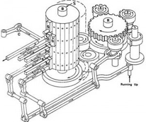
Back to multiplication. The engine needed an internal control mechanism to take it through this complex process and what it used was a microprogram encoded by pegs on a rotating barrel. You can see a simplified diagram of the barrel here on the right. Each “cycle” of the microprogram proceeds in the same way.

First the barrel is pushed left and the pegs along the vertical edge press against a row of levers which causes them to engage or disengage other parts of the engine. Because of the way the pegs are aligned with the vertical edge of the barrel Babbage called a single such instruction a vertical.

Second, the barrel is pushed to the right and connects to the big gear you see to the right of it in the diagram. That gear, and the gears connected with it, Babbage called the reducing apparatus. That’s what controls the flow of the program. The reducing apparatus rotates the barrel some amount in either direction to select the next vertical to apply. At the same time any other components that were engaged by the current vertical perform their operation, for instance a single step of building the multiplication table. The reducing apparatus takes input from those other components so for instance it may move the barrel different amounts depending on whether the last addition overflowed. That’s the arm on the far right (Babbage called overflow “running up”). The reducing apparatus is controlled by the barrel itself so each vertical explicitly specifies how the reducing apparatus should rotate it to the next vertical. You’ll notice that the three gears you see near the reducing apparatus’ main gear have 1, 2, and 4 teeth respectively. By engaging a combination of them one vertical could have the reducing apparatus rotate the barrel any number of steps between 1 to 7. In modern terms, each micro-instruction contains an explicit relative branch, conditional or unconditional, to the next microinstruction. As you can see this is a highly sophisticated and general mechanism. The only disadvantage is that it’s slow – a single cycle takes a few seconds so a multiplication can take several minutes.

As you would expect the diagram above is simplified, in practice there were multiple barrels and they were much larger both in the number of pegs for each vertical and number of verticals per drum. I haven’t been able to find any of Babbage’s actual microprograms unfortunately so for now all I know are the basic principles, and we know that designing them was one of Babbage’s main interests in designing the engine.

The third program format is the punched cards which is what would have been used by an operator of the engine. I’ll look at those in some detail because they give a good sense of what it would have been like to work with the engine in practice. To keep this post to a reasonable length I’ve broken that out into its own post called punched cards.

Difference

This is my second post in a series about Babbage’s mechanical calculating engines. The first post was about why it was so important in the early 1800s to be able to produce accurate arithmetic tables and ended with what I’ll be generous and call a cliffhanger: that Babbage’s difference engine was a groundbreaking solution to that problem. In this post I’ll explain how the difference engine works, how to “code” it and how to interpret what you get back.

Before we get to the engine itself there’s a bit of math to explain the basic principles it works by. To give you a taste of the engine itself before that here is a small JavaScript emulator1 that performs a simple calculation. It’s tiny compared to the real engine but works by the same principles just on a smaller scale.

Try stepping it a few times. The model is actually quite straightforward and the computations you can use it for are based on some basic mathematical principles. You can treat it as an exercise before reading the rest if you like: try to work out what it’s calculating, how it does it, and how you can make it calculate other things. Of course you can also just read on an I’ll tell you.

Differences

The difference engine is a very simple device in principle. It’s an adding machine, that’s all it is2. Part of what makes it such an impressive accomplishment is that it took a difficult problem, calculating complex functions, and solved it using a simple enough approach that it could be implemented mechanically using contemporary technology3.

So, how do you calculate complex functions using just addition? Obviously you can’t in general so let’s start off easy by looking just at polynomials.

Consider this simple polynomial, the square function:

f(x) = x^2

The first few values are

  \begin{tabular}{lcl}  f(0) & = & 0 \\  f(1) & = & 1 \\  f(2) & = & 4 \\  f(3) & = & 9 \\  & \vdots &  \end{tabular}

The difference engine is based on a technique called divided differences. Divided differences is similar to differentiation but simpler and it’s based on simple arithmetic. It works as follows. You take the values of your polynomial at a fixed interval, here we’ll use the first four values from before:

  \begin{tabular}{l}  0 \\  \\  1 \\  \\  4 \\  \\  9  \end{tabular}

Then you find the distance between each successive pair of them:

  \begin{tabular}{l|l}  0 \\  & 1 \\  1 \\  & 3 \\  4 \\  & 5 \\  9  \end{tabular}

These are the first differences. Then you find the distance between the first differences the same way:

  \begin{tabular}{l|l|l}  0 \\  & 1 \\  1 && 2\\  & 3 \\  4 && 2\\  & 5 \\  9  \end{tabular}

These are the second differences. And one last time to get the third differences:

  \begin{tabular}{l|l|l|l}  0 \\  & 1 \\  1 && 2\\  & 3 && 0\\  4 && 2\\  & 5 \\  9  \end{tabular}

You can see the similarity to differentiation: it’s a polynomial of degree 2 so the first differences increase linearly just like the first derivative, the second differences are constant just like the second derivative, and so on. We don’t actually need the third differences, they’ll all be 0 anyway, so I’ll leave those out below.

What’s neat is that once you have these values you can extend the table using nothing but addition. You know the difference between the first derivatives is fixed, 2, so you can get the next first derivative by adding 2 to the previous one. And you know the difference between the function values is the first differences so you can get the next value just by adding the next first difference to the previous function value. Okay maybe it’s easier to explain with a concrete example:

  \begin{tabular}{l|l|l}  0 \\  & 1 \\  1 && 2\\  & 3 \\  4 && 2 \\  & 5 \\  9  \end{tabular}  \quad\to\quad  \begin{tabular}{l|l|l}  0 \\  & 1 \\  1 && 2\\  & 3 \\  4 && 2 \\  & 5 & \tiny{+0} \\  9 && \bf{2}  \end{tabular}  \quad\to\quad  \begin{tabular}{l|l|l}  0 \\  & 1 \\  1 && 2\\  & 3 \\  4 && 2 \\  & 5 \\  9 & \tiny{+2} & \bf{2} \\  & \bf{7} \\  \end{tabular}  \quad\to\quad  \begin{tabular}{l|l|l}  0 \\  & 1 \\  1 && 2\\  & 3 \\  4 && 2 \\  & 5 \\  9 && \bf{2} \\  \tiny{+7} & \bf{7} \\  \bf{16} \\  \end{tabular}

Notice that we don’t need the full table at this point, we only need that for calculating the initial values. All we need to generate more values is the last of each of the differences:

  \begin{tabular}{l|l|l}  \multicolumn{1}{r}{}&&2 \\  & 7 & \tiny{+0}\\  16 &\tiny{+2}& 2 \\  \tiny{+9} & 9 \\  \bf{25} \\  \end{tabular}  \quad\to\quad  \begin{tabular}{l|l|l}  \multicolumn{1}{r}{}&&2 \\  & 9 & \tiny{+0}\\  25 &\tiny{+2}& 2 \\  \tiny{+11} & 11 \\  \bf{36} \\  \end{tabular}  \quad\to\quad  \begin{tabular}{l|l|l}  \multicolumn{1}{r}{}&&2 \\  & 11 & \tiny{+0}\\  36 &\tiny{+2}& 2 \\  \tiny{+13} & 13 \\  \bf{49} \\  \end{tabular}  \quad\to\quad\dots

This provably works for any polynomial. To generate a sequence of values for a polynomial of degree n all you need is n+1 initial values; from the values you calculate the table of differences using subtraction, and from there on you can calculate as many successive values as you like using just addition. You don’t even need to know the closed form of the polynomial as long as you can evaluate the initial values at fixed intervals.

This is the basic principle of the difference engine, and what it’s named after. The engine has 8 integer registers called columns that can each hold a 31-digit integer value which represent the current value of the function and the first to the seventh difference. By cranking the handle those values are added together from right to left. Here is a another mini-emulator, this one calculating the square function using the differences we just calculated:

You can see the values are being added together from right to left and the current function value in the leftmost column is printed for each emulated crank on the handle. Printing was also a part of the original difference engine. A common source of errors in mathematical tables was typesetting so to avoid that step the engine would automatically stamp its output in a soft material that could be used directly for printing, as well as print a log on paper.

Being able to evaluate an integer polynomial is just the beginning though. First of all, integers aren’t enough, we need to be able to evaluate real-valued functions. Secondly, so far we’ve only seen positive values, we also need negatives. Finally, polynomials can be useful in themselves but we’re really more interested in more complex functions like logarithms and trigonometric or astronomical functions. But with a few tricks the difference engine can handle all those things.

Precision

First off: how do we use this to evaluate real-valued functions? You use fixed-point decimal numbers. For instance, say we want to plot the square function from before but this time in steps of 0.25:

  \begin{tabular}{lcl|l|l}  f(0) & = & 0 \\  &&& 0.0625 \\  f(0.25) & = & 0.0625 && 0.125 \\  &&& 0.1875 \\  f(0.5) & = & 0.25  \end{tabular}

These are fractional numbers but if you multiply them by 105 we’re back to integers

  \begin{tabular}{lcl|l|l}  10000 f(0) & = & 0 \\  &&& 625 \\  10000 f(0.25) & = & 625 && 1250 \\  &&& 1875 \\  10000 f(0.5) & = & 2500 \\  \end{tabular}

Now we’re back to something the engine can calculate:

I’ve added a line between the digits to mark where the decimal point goes. It also gets added to the output (I don’t believe the original engine did this). But the decimal point is purely a matter of interpretation by the operator, the adding mechanism is not aware of it, it’s operating purely on 6-digit integer values.

In this case we were lucky because there was a relatively small factor of 10 we could multiply onto the values to get integers without losing precision. That’s unlikely to be the case in general. If you can’t use this trick you multiply the values with as large a factor of 10 as you have precision for and just bite the bullet, round the scaled values to the nearest integers and lose some accuracy. That’s not necessarily as bad as it sounds. The original design had 31 digit precision in base 10 which corresponds to roughly 103 bits, well beyond the already quite large 64-bit integers on most modern machines. So you can afford to scale the values up quite a bit before rounding. We’ll see an example in a bit of how long it takes for errors to accumulate.

Negative values

To represent negative values we use the exact same trick as with binary numbers, just in base 10: tens complement. A negative number d is represented as 10n – d where n is the number of decimal digits, so -1 is represented by 999…999 and so forth. The adding mechanism itself has no concept of negative values, just like with twos complement the correct behavior just falls out of how overflow works. It’s up to the operator or printer to interpret the output correctly as signed or unsigned values.

Here is an example of a function that starts off positive, peaks, and then descends into the negative numbers.

You’ll notice that the numbers in the columns are all positive but the ones that represent negative values are printed as negative. As with the decimal point that’s a hack I added in the printer which makes it print smaller integer values as positive and larger ones as negative. But it’s purely a matter of interpretation, the calculating part of the engine is oblivious.

Polynomial approximation

Okay, now we’re getting close to the goal: being able to produce accurate arithmetic tables of general functions.

In my previous post the main example of how important mathematical tables were was how astronomical tables were used by mariners to navigate by lunar distance. I don’t actually know the math underlying those astronomical tables so here I’ll use an example I do understand: trigonometric functions. On the right here is a table of trigonometric functions from 1785. It gives 7 digits of the values of 8 different trignonmetric functions, sin, cos, tan, etc., for each arcminute between 0° and 45°. There’s 60 arcminutes to one degree so that’s 2700 values for each function, 21,600 values in total. The author of this table, Charles Hutton, said about this edition in a later one that it had so many errors that is was basically useless:

Finding, as well from the report of others, as from my own experience, that those editions […] were so very incorrectly printed, the errors being multiplied beyond all tolerable bounds, and no dependence to be placed on them for any thing of real practice […]

For this last part about how to calculate complex functions I’ll show how to replicate one column, sin, of this table.

Since we know how to evaluate polynomials the solution that first springs to mind is to approximate the function we want to calculate using a polynomial. Taylor polynomials were well known at this time so that’s an obvious approach. Taylor’s theorem says that for an infinitely differentiable function f (which sin is),

f(x) = \sum_{k=0}^{\infty}\frac{f^{(k)}(a)}{k!}(x-a)^k

where f(k) means f differentiated n times and a is any point on the function. Since the engine only has 8 columns and we need n+1 columns for a polynomial of degree n we have to limit ourselves to at most the first 7 terms. And in fact, since I want to demonstrate this with the emulator in a little bit and 8 columns of 31 digits takes up an enormous amount of space we’ll limit ourselves even more in this example to 4 columns of 13 digits. This means that we’ll use only the first 3 terms of the Taylor polynomial. For sin those are:

\sin(x) \approx x - \frac{x^3}{3!}

(Conveniently all the even degree terms are 0). This approximates sin quite well around 0 so we’ll use that as the basis for generating the table.

To calculate the differences we first need to produce n+1 values at fixed intervals. The generated table should have an entry per arcminute so we’ll start at 0′ and do steps of 1′:

x sin(x)
0′ 0
1′ 2.909 10-4
2′ 5.818 10-4
3′ 8.727 10-4

Then we need to find the nth differences:

x sin(x) Δ1 Δ2 Δ3
0′ 0 2.909 10-4 -2.461 10-11 -2.461 10-11
1′ 2.909 10-4 2.909 10-4 -4.923 10-11
2′ 5.818 10-4 2.909 10-4
3′ 8.727 10-4

All of this is a matter of evaluating a polynomial so that’s not super hard to do by hand with as many decimals as you need, as long as you only need a few of them. From this table we take the last of each of the differences and that’ll be the starting point for the calculation:

0.000872664515235
0.000290888130722
-0.000000000049228
-0.000000000024614

At this point we need to decide how much accuracy we want, that is, where we want the fixed decimal point to be. We have 13 digits which gives us room enough to multiply by 1013 before rounding. That gives us these integer values:

8726645152
2908881307
-492
-246

And now we’re ready to get tabulating:

If you follow along with the original table you can see that it generates exactly the same values. The values generated by the engine continue to match the table values until 1° 1′, 57 values in, where the table says 0.0177432 and the engine produces 0.0177433, and after that it continues to produce matching values up until 1° 53′, more than 100 values in.

Not bad right? And remember, this is a simplified emulator that can only calculate the third degree approximation where the original could go up to the seventh, and only with 13 digits of precision where the original had 31.

So what’s the source of the deviation? There’s two: the approximating polynomial and the accumulating error of the engine. Let’s first look at the polynomials.

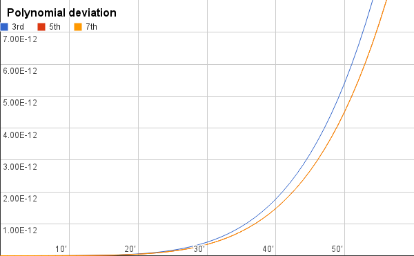
The first plot on the right is of how quickly the approximating polynomials of different degrees deviate from the true sine function. At 1° the approximations are still well within 0.01 billionth of the correct value. Like I said, near 0 these polynomials approximate sin really well.

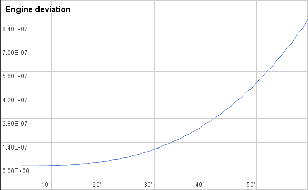
This suggests that the main source of inaccuracy is the engine itself, the precision we had to discard when fixing the decimal point, and as you can see in the second graph, it is. The engine loses precision faster than the polynomial by a large factor. This makes sense because the inaccuracy accumulates for every step.

Luckily in this case the polynomial deviates slowly enough we can use it to calculate new almost-accurate initial values at fixed intervals, for instance for each degree, and reset the machine to those. However, eventually the polynomial itself will deviate too much and at that point we can use the fact that the Taylor polynomial has an a parameter that specifies the point around which we’re approximating. So say the polynomial that approximates around 0° becomes too inaccurate at 6° we can derive a Taylor polynomial around 6° and use that to continue the calculation. Indeed, since the polynomial approximates equally well on both sides of the point we might as well approximate around 9° and use it for all values between 6° and 12°.

Sin is a relatively easy function to approximate in this way, a function such as log is harder but the same basic principles apply to harder functions. It’s a matter of how often you need to reset to get rid of the accumulating errors and how long the same approximating polynomial remains accurate.

One of the weak points of the engine is that even though it requires less manual work than producing a table completely manually, there’s still a fair amount of manual analysis and computation to be done. That’s not a killer in itself though. Even if it took just as much work to operate, which it surely wouldn’t have, just having a different way to create these tables would have been immensely valuable since two different approaches are likely to produce different errors and hence can be used to cross-check each other. But as this illustrates, even if the engine had been built it was definitely not a matter of just plugging in a few values and then going to lunch, using it involved a fair amount of work4.

The revolution that didn’t happen

Here’s a video of the only difference engine ever built which was completed in 2002.

Babbage tried to build it and ultimately gave up for a number of reasons including family problems, financial problems, problems working with his engineer, and his gradual change of focus to the analytical engine. Despite what you often hear the technology did exist to build it; the modern one was built from his designs and only with technology that would have been available back then.

It also appears that Babbage’s interests and those of the English government who paid for the whole thing were just too far apart. Babbage was interested in the machine itself whereas his sponsors just wanted accurate tables, whatever way Babbage could produce them. It’s a shame really. It seems from what I’ve read that the difference engine was a failure not of vision or technology but of product management. The technology was so promising that if a successful prototype had been built and he’d delivered the tables the English government wanted it’s not unlikely that they would have continued to fund research in more advanced engines. The ground would have been fertile for mechanical calculation on a larger scale by the mid 1800s. Obviously that wouldn’t have meant a mechanical iPad in every home by 1900 but it would certainly have been a better outcome than what happened, that the designs went in the drawer.

Ultimately Babbage moved on to the analytical engine, the first ever programmable computer. My next post will be about that and in particular the first ever software programs which were written for it.

Sources

For more information about the difference engine a quick introduction is given in the first part of Menabrea’s Sketch of the Analytical Engine from 1842. A more detailed description, including of the underlying mechanics of the engine, can be found in Lardner’s Babbage’s Calculating Engine from the July 1834 edition of the Edinburgh Review.

Notes

1: While the emulator performs the same type of calculations as the difference engine it actually looks nothing like it. I made a point to give the emulator a mechanical feel but it’s inspired more by the Curta calculator, the mechanical calculator I know best, not the difference engine. Note also that I have only tested it on the browsers I have easy access to, Chrome, Firefox, Opera, and Safari on mac. If it doesn’t work on your platform the code lives on github and patches are welcome.

2: Ada Lovelace in her famous notes about it is almost contemptuous of how simple it is compared to the analytical engine:

The Difference Engine can in reality […] do nothing but add; and any other process […] can be performed by it only just to the extent in which it is possibly, by judicious mathematical arrangement and artifices, to reduce them to a series of additions.

3: Incidentally, much of the underlying math was developed before Babbage by J. H. Müller.

4: I wonder if it’s possible to automate some of the manual work involved in operating the engine using the engine itself, like calculating initial values.

Tables

I have a thing for mechanical calculators and it recently occurred to me that I knew almost nothing about two of the most famous ones: Babbage’s difference engine and analytical engine. This led me to read some of the papers from the mid 1800s that were written about them. This blog post is the first of a few I’m planning to write about that.

The analytical engine usually gets most of the attention but the difference engine is an interesting invention in its own right. Not only did it solve an important problem, it is the only one of the two that was complete enough to actually be built. This post about what made the difference engine so important that Babbage spent decades trying to build it and why British government was willing to pay the bill of over ₤17,000, more than the price of two warships.

Calculation

Today computation is cheap. Extremely cheap. Imagine the amount of math that goes into just displaying the image on your screen right now: the layouts, colors, and fonts, rendering it all on a physical display, and doing it again and again quickly and smoothly enough that you don’t even notice it’s happening.

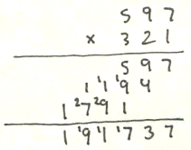
Computation is so cheap that it’s easy to forget how expensive it was before electronic calculators. It used to be that if you wanted to add two numbers together you had to actually add those numbers together. Manually. Need to multiply or divide two numbers, even just a few digits? Then you’ll have to get the paper out and do long multiplication or long division. I just did a long multiplication to make the image on the right here. I got it wrong twice before getting it right and I went from “this’ll be fun, I wonder if I still remember how to do this” to “god this is so tedious” in about 30 seconds.

And those are just the basic building blocks of doing a calculation. Most interesting computations like calculating interest or the position of the moon in six months require you to do these manual computations over and over and over again. Or require operations that you can’t easily calculate by hand, like trigonometric functions.

At this point you might be thinking: who cares where the moon is in six months? It turns out, back in those days a lot of people did. In some cases people’s lives depended on it.

Lunar Navigation

On the right here is a table of distances in degrees on the night sky from the center of the moon to various stars at particular times. The first line gives the distance between the center of the moon and Aldebaran on March 3, 1775 at noon, 3, 6, and 9 o’clock. Multiply that by 365 days, then multiply it by a dozen stars, that gives you just some of the tables in this book, the first edition of the Nautical Almanc and Astronomical Ephemeris from 1774, published from the Royal Greenwich Observatory. The audience for the almanac were mariners. The first edition of 10,000 copies sold out immediately.

To determine your longitude at sea you need to know the current time at a fixed point. You can think of it sort of like navigating with time zones. If you know it’s 4 o’clock in the afternoon Greenwich and it’s noon where you are (which you can tell by looking at the sun) then you know you’re in the -4 time zone which is the one that goes through eastern Canada, the eastern Caribbean and central South America. This is a rough analogy but that’s the gist of how it works.

Up until around 1850, before accurate clocks were made that could be carried on long voyages, a reliable way to determine the current time was using lunar distance. The moon and stars in the night sky move as a perfectly predictable clockwork. A given configuration occurs only once, and you can calculate in advance precisely what the sky is going to look like at a later time. And more importantly you can go the other way: given the precise configuration of the sky you can calculate exactly what time it is.

Actually you don’t need the full configuration; all you need to know to calculate the time is the distance in degrees from the center of the moon to any star. That’s where the almanac comes in. It precomputes those distances so that all a navigator needs to do is measure the angle (typically using a sextant) and then look the value up in the almanac. Okay that’s actually just the basic principle, there’s a lot more to it in practice: you have to adjust for the distance from the center of the moon to the circumference, for your position on the earth, for atmospheric refraction, etc. Being a navigator takes a lot of skill. How do you make those adjustments by the way? More tables of course.

All this means that having accurate tables is extremely important. An undetected error in the almanac means a navigation error which can mean shipwreck. This is made worse because many of these tables are time dependent: one line in the almanac is useful on one day only. As a navigator you’re basically beta testing the data for every single day because nobody has had any reason to use the data before.

There are many sources of errors in numerical tables. Teams of human computers carried out the manual calculations, a tedious and error prone process. (Incidentally, it turns out that the better an understand you have of the calculation you’re carrying out the more likely you are to make mistakes as a computer.) Often the same value would be calculated by more than one human computer and then compared to catch errors – but checking is an error prone process in itself, and computers can (and did) copy from each other. Then finally someone has to manually set the values in movable type and print them, also an obvious source of errors.

Enter Charles Babbage.

Babbage

Babbage was an unorthodox and very gifted mathematician. He was a fan of Leibniz which was still something of a heresy at his college Trinity, home of Newton, Leibniz’s arch rival. He was also one of the founders of the Analytical Society whose goal it was to replace Newton’s formalism for calculus with Leibniz’s. Incidentally, besides inventing calculus independently from Newton Leibniz designed a mechanical calculating machine, the stepped reckoner.

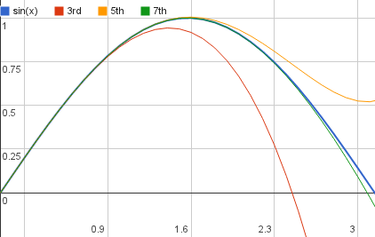
Babbage recognized the problem of calculating tables, as most people did, but also had a solution: the difference engine. The idea behind the difference engine is that most of the functions you want to create tables for can be approximated by a polynomial. Here is the sine function along with three approximating polynomials of increasing degree:

As the degree of the polynomial increases the approximation quickly becomes better – the degree-seven polynomial is quite close:

f_7(x) = x - \frac{x^3}{3!} + \frac{x^3}{5!} - \frac{x^7}{7!}

Babbage’s idea was to use mechanical means to calculate the approximating polynomials with high accuracy not just print the result on paper but do the actual typesetting to eliminate even the typographer as a source of errors.

But I’ll stop here before we get to the juicy details of how the difference engine works and save that for my next blog post.