Category Archives: mathematics

Making tea

This post is about the mathematics of making a good cup of tea. I drink a lot of tea and for a long time I would ignore the direction to use water below boiling, say 75° or 85°. Because – if you don’t have a boiler with a temperature setting how do you get water at less than 100°? Wait for it to cool? Come on!

Of course you can do it easily by adding cold water, you just have to figure out how much. While I was waiting for a delivery this morning I thought I’d look into that and it turned out to be a fun little practical application of the scientific method.

Theory 1: the average temperature

Let’s assume tap water is 22° and you add 500ml of it to the same amount of boiling water. My starting assumption was that the result will be 1l of water at the average of the two temperatures, 61°:

t_r = \frac{100 \cdot 500 + 22 \cdot 500}{500 + 500}=61

Put more generally, my theory was that if you mix water of two different temperatures then the temperature of the result will be the average over the two temperatures, where each temperature is weighted by the volume of water

t_r = \frac{100 v_b + t_t v_t }{v_b + v_t}

(Here t_r is the resulting temperature of the water, v_b is the amount of boiling water which will be 100°, t_t is the temperature of tap water, and v_t is the amount of tap water.)

If you measure the tap water temperature and know how much water your tea pot will hold you can solve for the amount of boiling and tap water to use to make any given water temperature. For instance, my tap water is 22° and my tea pot holds 700ml so the formula for how much to boil for a given temperature is,

t_r = \frac{100 v_b + 22 (700 - v_b)}{700}

t_r = \frac{100 v_b + 22 \cdot 700 - 22 v_b}{700}

t_r = \frac{78 v_b + 22 \cdot 700}{700}

700 (t_r - 22) = 78 v_b

\frac{700}{78} (t_r - 22) = v_b

So to get a pot full of 85° water, the amount of boiling water should be

\frac{700}{78} (85 - 22) = 8.97 \cdot 63 = 565

Boil 565ml, add the rest up to 700ml from the tap (that would be 135ml) and you’ve got 700ml of 85° water. That’s the theory.

Ok, so having solved the problem I went to make tea, my delivery having still not arrived (spoiler alert: it arrived while I was at the dentist, obviously). It turns out though that the theory doesn’t work. When I did it in practice it turned out that the water wasn’t 85°, it was 77°. Bummer. The theory is too simplistic.

Theory 2: the tea pot constant

The problem was fortunately obvious: I was pouring the water into a cold tea pot. The formula only says what happens to the water itself, it doesn’t take into account that it all ends up in a pot that’s initially at room temperature.

What I thought I’d do then was to model the effect of the cold pot as if it were extra tap water. How much exactly I don’t know, but it seems reasonable to expect that the cooling effect of a particular pot works basically the same way as if you’d added a bit of extra cold water. So we replace v_t in the formula above, the amount of tap water, with v_t + v_p, the amount of tap water and some additional amount, v_p, to account for the pot,

t_r = \frac{100 v_b + t_t (v_t + v_p) }{v_b + v_t + v_p}

You have to determine v_p experimentally, it is a property of a particular pot just like the volume. I determined it by pouring boiling water into the cool pot and then measuring the temperature; it had dropped to 90°. Using this I could find v_p,

t_r = \frac{100 v_b + t_t (v_t + v_p) }{v_b + v_t + v_p}

90 = \frac{100 \cdot 700 + 22 (0 + v_p) }{700 + v_p}

90 \cdot 700 + 90 v_p = 100 \cdot 700 + 22 v_p

-10 \cdot 700 = -68 v_p

\frac{10 \cdot 700}{68} = v_p = 103

In other words: the pot cools boiling water as much as adding 103ml of extra tap water.

Again, it’s just a theory that this makes sense, but it’s a theory we can test. Earlier, I mixed 565ml boiling and 135ml tap water and got 77° instead of the 85° I expected. What does the new theory predict will happen?

t_r = \frac{100 v_b + t_t (v_t + v_p) }{v_b + v_t + v_p}

t_r = \frac{100 \cdot 565 + 22 \left( 135 + 103 \right) }{700 + 103} = 76.9

That’s so close to the 77° that you’d almost think I fudged the numbers, but it’s really just a coincidence.

With this new and more plausible general formula we can plug in the values for my pot and water and get a specific formula for how much boiling and tap water to use to produce a particular temperature in my pot,

t_r = \frac{100 v_b + 22 (700 - v_b + 103)}{700 + 103}

t_r = \frac{100 v_b + 22 \cdot 803 - 22 v_b}{803}

t_r = \frac{78 v_b + 22 \cdot 803}{803}

803 (t_r - 22) = 78 v_b

\frac{803}{78} (t_r - 22) = v_b

It turns out to be the same as the one before except with 803 instead of 700. Using this formula, then, to get 85° water I need

\frac{803}{78} (85 - 22) = 10.29 \cdot 63 = 648

ml of boiling and the rest, 52ml, of tap. I tried this out and the result was… drumroll… 86°. So the formula seems to work. Yay!

Summary

So, to sum all this up, here’s how you apply the formulas in practice.

Measure how much water it takes to fill your pot, call that v. Boil that much water and pour it into the pot. Measure the temperature and call that t_p. Measure the temperature of your tap water, call that t_t. Plug them into this formula to get the tea pot constant for your tea pot, v_p

v_p = v \frac{t_p - 100}{t_t - t_p}

Then, given a temperature t_r, the amount of water to boil to get that temperature can be calculated by,

v_b = \frac{(v+v_p) (t_r-t_t)}{100-t_t}

And that’s it. You only have to calculate these once for a given pot so even though it’s a hassle, it’s a one time hassle. And it’s possible that most tea pots have approximately the same constant, in which case you can just assume that yours has the same one. But that’s for future research into the fertile field that is the science of tea.

Ironically, I got so caught up calculating the ideal amount of water that I never actually made tea, just water of different temperatures. I think I’ll go make some actual tea now.

Radix

Over on my tumblr I’ve been having a bit of fun with number systems. The first post is about how the claim that e is the most efficient radix is wrong, and the other is about how you can use a non-integer, for instance e, can be made to work a radix.

0x5f3759df (appendix)

This post is an appendix to my previous post about 0x5f3759df. It probably won’t make sense if you haven’t read that post (and if you’ve already had enough of  0x5f3759df you may consider skipping this one altogether).

One point that bugged me about the derivation in the previous post was that while it explained the underlying mathematics it wasn’t very intuitive. I was basically saying “it works because of, umm, math“. So in this post I’ll go over the most abstract part again (which was actually the core of the argument). This time I’ll explain the intuition behind what’s going on. And there’ll be some more graphs. Lots of them.

The thing is, there is a perfectly intuitive explanation for why this works. The key is looking more closely at the float-to-int bit-cast operation. Let’s take that function,

int float_to_int(float f) {
  return *(int*)&f;
}

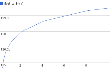
and draw it as a graph:

This is a graph of the floating-point numbers from around 1 to 10 bit-cast to integers. These are very large integers (L is 223 so 128L is 1 073 741 824). The function has visible breaks at powers of two and is a straight line inbetween. This makes sense intuitively if you look at how you decode a floating-point value:

v = (1+m)2^e

The mantissa increases linearly from 0 to 1; those are the straight lines. Once the mantissa reaches 1 the exponent is bumped by 1 and the mantissa starts over from 0. Now it’ll be counting twice as fast since the increased exponent gives you another factor of 2 multiplied onto the value. So after a break the straight line covers twice as many numbers on the x axis as before.

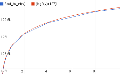
Doubling the distance covered on the x axis every time you move a fixed amount on the y axis – that sounds an awful lot like log2. And if you plot float_to_int and log2 (scaled appropriately) together it’s clear that one is an approximation of the other.

In other words we have that

\mathtt{float\_to\_int}(v) \approx (\log_2(v)+B)L

This approximation is just a slightly different way to view the linear approximation we used in the previous post. You’ll notice that the log2 graph overshoots float_to_int in most places, they only touch at powers of 2. For better accuracy we’ll want to move it down a tiny bit – you’ll already be familiar with this adjustment: it’s σ. But I’ll leave σ out of the following since it’s not strictly required, it only improves accuracy.

You can infer the approximation formula from the above formula alone but I’ll do it slightly differently to make it easier to illustrate what’s going on.

The blue line in the graph above,  float_to_int(v), is the i in the original code and the input to our calculation. We want to do integer arithmetic on that value such we get an output that is approximately

\mathtt{float\_to\_int}(v^{-\frac 12})

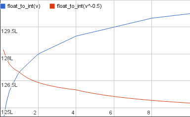
the integer value that, if converted back to a float, gives us roughly the inverse square root of x. First, let’s plot the input and the desired output in a graph together:

The desired output is decreasing because it’s a reciprocal so the larger the input gets the smaller the output. They intersect at v=1 because the inverse square root of 1 is 1.

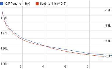
The first thing we’ll do to the input is to multiply it by -1 to make it decrease too:

Where before we had a very large positive value we now have is a very large negative one. So even though they look like they intersect they’re actually very far apart and on different axes: the left one for the desired output, the right one for our work-in-progress approximation.

The new value is decreasing but it’s doing it at a faster rate than the desired output. Twice as fast in fact. To match the rates we multiply it by 1/2:

Now the two graphs are decreasing at the same rate but they’re still very far apart: the target is still a very large positive value and the current approximation is a half as large negative value. So as the last step we’ll add 1.5LB to the approximation, 0.5LB to cancel out the -1/2 we multiplied it with a moment ago and 1LB to bring it up to the level of the target:

And there it is: a bit of simple arithmetic later and we now have a value that matches the desired output:

\mathtt{float\_to\_int}(v^{-\frac 12}) \approx \frac 32LB - \frac 12 \mathtt{float\_to\_int}(v)

The concrete value of the constant is

\frac 32LB = \mathtt{0x5f400000}

Again the approximation overshoots the target slightly the same way the log2 approximation did before. To improve accuracy you can subtract a small σ from B. That will give a slightly lower constant – for instance 0x5f3759df.

And with that I think it’s time to move onto something else. I promise that’s the last you’ll hear from me on the subject of that constant.

0x5f3759df

This post is about the magic constant 0x5f3759df and an extremely neat hack, fast inverse square root, which is where the constant comes from.

Meet the inverse square root hack:

float FastInvSqrt(float x) {
  float xhalf = 0.5f * x;
  int i = *(int*)&x;         // evil floating point bit level hacking
  i = 0x5f3759df - (i >> 1);  // what the fuck?
  x = *(float*)&i;
  x = x*(1.5f-(xhalf*x*x));
  return x;
}

What this code does is calculate, quickly, a good approximation for

\frac{1}{\sqrt{x}}

It’s a fairly well-known function these days and first became so when it appeared in the source of Quake III Arena in 2005. It was originally attributed to John Carmack but turned out to have a long history before Quake going back through SGI and 3dfx to Ardent Computer in the mid 80s to the original author Greg Walsh. The concrete code above is an adapted version of the Quake code (that’s where the comments are from).

This post has a bit of fun with this hack. It describes how it works, how to generalize it to any power between -1 and 1, and sheds some new light on the math involved.

(It does contain a fair bit of math. You can think of the equations as notes – you don’t have to read them to get the gist of the post but you should if you want the full story and/or verify for yourself that what I’m saying is correct).

Why?

Why do you need to calculate the inverse of the square root – and need it so much that it’s worth implementing a crazy hack to make it fast? Because it’s part of a calculation you do all the time in 3D programming. In 3D graphics you use surface normals, 3-coordinate vectors of length 1, to express lighting and reflection. You use a lot of surface normals. And calculating them involves normalizing a lot of vectors. How do you normalize a vector? You find the length of the vector and then divide each of the coordinates with it. That is, you multiply each coordinate with

\frac{1}{\sqrt{x^2+y^2+z^2}}

Calculating x^2+y^2+z^2 is relatively cheap. Finding the square root and dividing by it is expensive. Enter FastInvSqrt.

What does it do?

What does the function actually do to calculate its result? It has 4 main steps. First it reinterprets the bits of the floating-point input as an integer.

int i = *(int*)&x;         // evil floating point bit level hack

It takes the resulting value and does integer arithmetic on it which produces an approximation of the value we’re looking for:

i = 0x5f3759df - (i >> 1);  // what the fuck?

The result is not the approximation itself though, it is an integer which happens to be, if you reinterpret the bits as a floating point number, the approximation. So the code does the reverse of the conversion in step 1 to get back to floating point:

x = *(float*)&i;

And finally it runs a single iteration of Newton’s method to improve the approximation.

x = x*(1.5f-(xhalf*x*x));

This gives you an excellent approximation of the inverse square root of x. The last part, running Newton’s method, is relatively straightforward so I won’t spend more time on it. The key step is step 2: doing arithmetic on the raw floating-point number cast to an integer and getting a meaningful result back. That’s the part I’ll focus on.

What the fuck?

This section explains the math behind step 2. (The first part of the derivation below, up to the point of calculating the value of the constant, appears to have first been found by McEniry).

Before we can get to the juicy part I’ll just quickly run over how standard floating-point numbers are encoded. I’ll just go through the parts I need, for the full background wikipedia is your friend. A floating-point number has three parts: the sign, the exponent, and the mantissa. Here’s the bits of a single-precision (32-bit) one:

s e e e e e e e e m m m m m m m m m m m m m m m m m m m m m m m

The sign is the top bit, the exponent is the next 8 and the mantissa bottom 23. Since we’re going to be calculating the square root which is only defined for positive values I’m going to be assuming the sign is 0 from now on.

When viewing a floating-point number as just a bunch of bits the exponent and mantissa are just plain positive integers, nothing special about them. Let’s call them E and M (since we’ll be using them a lot). On the other hand, when we interpret the bits as a floating-point value we’ll view the mantissa as a value between 0 and 1, so all 0s means 0 and all 1s is a value very close to but slightly less than 1. And rather than use the exponent as a 8-bit unsigned integer we’ll subtract a bias, B, to make it a signed integer between -127 and 128. Let’s call the floating-point interpretation of those values e and m. In general I’ll follow McEniry and use upper-case letters for values that relate to the integer view and and lower-case for values that relate to the floating-point view.

Converting between the two views is straightforward:

m = \frac{M}{L}

e = E - B

For 32-bit floats L is 223 and B is 127. Given the values of e and m you calculate the floating-point number’s value like this:

(1+m)2^e

and the value of the corresponding integer interpretation of the number is

M + LE

Now we have almost all the bits and pieces I need to explain the hack so I’ll get started and we’ll pick up the last few pieces along the way. The value we want to calculate, given some input x, is the inverse square root or

y = \frac{1}{\sqrt{x}} = x^{-\frac 12}

For reasons that will soon become clear we’ll start off by taking the base 2 logarithm on both sides:

\log_2 y = {-\frac 12}\log_2 x

Since the values we’re working with are actually floating-point we can replace x and y with their floating-point components:

\log_2 (1+m_y) + e_y = {-\frac 12}(\log_2 (1+m_x) + e_x)

Ugh, logarithms. They’re such a hassle. Luckily we can get rid of them quite easily but first we’ll have to take a short break and talk about how they work.

On both sides of this equation we have a term that looks like this,

\log_2(1 + v)

where v is between 0 and 1. It just so happens that for v between 0 and 1, this function is pretty close to a straight line:
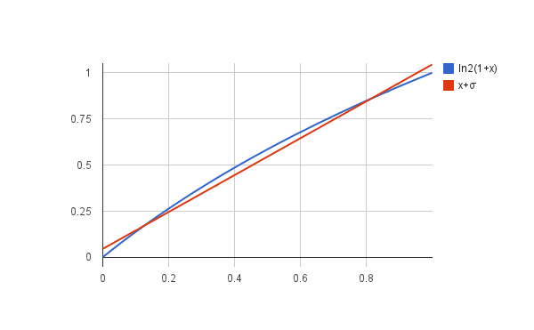
ln2(1 + x) vs. x + sigma

Or, in equation form:

\log_2(1 + v) \approx v + \sigma

Where σ is a constant we choose. It’s not a perfect match but we can adjust σ to make it pretty close. Using this we can turn the exact equation above that involved logarithms into an approximate one that is linear, which is much easier to work with:

m_y + \sigma + e_y \approx {-\frac 12}(m_x + \sigma + e_x)

Now we’re getting somewhere! At this point it’s convenient to stop working with the floating-point representation and use the definitions above to substitute the integer view of the exponent and mantissa:

\frac{M_y}{L} + \sigma + E_y - B \approx {-\frac 12}(\frac{M_x}{L} + \sigma + E_x - B)

If we shuffle these terms around a few steps we’ll get something that looks very familiar (the details are tedious, feel free to skip):

\frac{M_y}{L} + E_y \approx {-\frac 12}(\frac{M_x}{L} + \sigma + E_x - B) - \sigma + B

\frac{M_y}{L} + E_y \approx {-\frac 12}(\frac{M_x}{L} + E_x) - \frac{3}{2}(\sigma - B)

M_y + LE_y \approx {\frac 32}L(B - \sigma) - {\frac 12}(M_x + LE_x)

After this last step something interesting has happened: among the clutter we now have the value of the integer representations on either side of the equation:

\mathbf{I_y} \approx {\frac 32}L(B - \sigma) - {\frac 12}\mathbf{I_x}

In other words the integer representation of y is some constant minus half the integer representation of x. Or, in C code:

i = K - (i >> 1);

for some K. Looks very familiar right?

Now what remains is to find the constant. We already know what B and L are but we don’t have σ yet. Remember, σ is the adjustment we used to get the best approximation of the logarithm, so we have some freedom in picking it. I’ll pick the one that was used to produce the original implementation, 0.0450465. Using this value you get:

{\frac 32}L(B - \sigma) = {\frac 32}2^{23}(127 - 0.0450465) = 1597463007

Want to guess what the hex representation of that value is? 0x5f3759df. (As it should be of course, since I picked σ to get that value.) So the constant is not a bit pattern as you might think from the fact that it’s written in hex, it’s the result of a normal calculation rounded to an integer.

But as Knuth would say: so far we’ve only proven that this should work, we haven’t tested it. To give a sense for how accurate the approximation is here is a plot of it along with the accurate inverse square root:
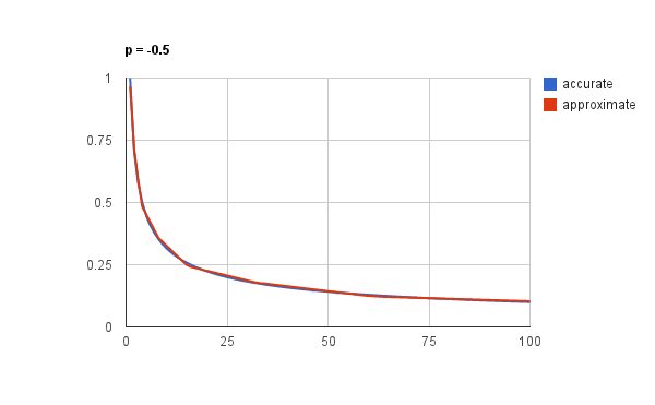
Graph of approximation vs. accurate value

This is for values between 1 and 100. It’s pretty spot on right? And it should be – it’s not just magic, as the derivation above shows, it’s a computation that just happens to use the somewhat exotic but completely well-defined and meaningful operation of bit-casting between float and integer.

But wait there’s more!

Looking at the derivation of this operation tells you something more than just the value of the constant though. You will notice that the derivation hardly depends on the concrete value of any of the terms – they’re just constants that get shuffled around. This means that if we change them the derivation still holds.

First off, the calculation doesn’t care what L and B are. They’re given by the floating-point representation. This means that we can do the same trick for 64- and 128-bit floating-point numbers if we want, all we have to do is recalculate the constant which it the only part that depends on them.

Secondly it doesn’t care which value we pick for σ. The σ that minimizes the difference between the logarithm and x+σ may not, and indeed does not, give the most accurate approximation. That’s a combination of floating-point rounding and because of the Newton step. Picking σ is an interesting subject in itself and is covered by McEniry and Lomont.

Finally, it doesn’t depend on -1/2. That is, the exponent here happens to be -1/2 but the derivation works just as well for any other exponent between -1 and 1. If we call the exponent (because e is taken) and do the same derivation with that instead of -1/2 we get:

\mathbf{I_y} \approx (1 - p)L(B - \sigma) + p\mathbf{I_x}

Let’s try a few exponents. First off p=0.5, the normal non-inverse square root:

\mathbf{I_y} \approx K_{\frac 12} + {\frac 12}\mathbf{I_x}

K_{\frac 12} = {\frac 12}L(B - \sigma) = {\frac 12}2^{23}(127 - 0.0450465) = \mathtt{0x1fbd1df5}

or in code form,

i = 0x1fbd1df5 + (i >> 1);

Does this work too? Sure does:
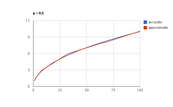
Graph of approximation vs. accurate

This may be a well-known method to approximate the square root but a cursory google and wikipedia search didn’t suggest that it was.

It even works with “odd” powers, like the cube root

\mathbf{I_y} \approx K_{\frac 13} + {\frac 13}\mathbf{I_x}

K_{\frac 13} = {\frac 23}L(B - \sigma) = {\frac 23}2^{23}(127 - 0.0450465) = \mathtt{0x2a517d3c}

which corresponds to:

i = (int) (0x2a517d3c + (0.333f * i));

Since this is an odd factor we can’t use shift instead of multiplication. Again the approximation is very close:
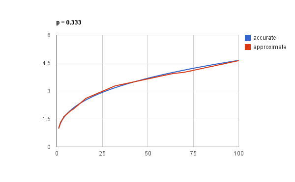
Graph of approximation vs. accurate

At this point you may have noticed that when changing the exponent we’re actually doing something pretty simple: just adjusting the constant by a linear factor and changing the factor that is multiplied onto the integer representation of the input. These are not expensive operations so it’s feasible to do them at runtime rather than pre-compute them. If we pre-multiply just the two other factors:

L(B - \sigma) = 2^{23}(127 - 0.0450465) = \mathtt{0x3f7a3bea}

we can calculate the value without knowing the exponent in advance:

i = (1 - p) * 0x3f7a3bea + (p * i);

If you shuffle the terms around a bit you can even save one of multiplications:

i = 0x3f7a3bea + p * (i - 0x3f7a3bea);

This gives you the “magic” part of fast exponentiation for any exponent between -1 and 1; the one piece we now need to get a fast exponentiation function that works for all exponents and is as accurate as the original inverse square root function is to generalize the Newton approximation step. I haven’t looked into that so that’s for another blog post (most likely for someone other than me).

The expression above contains a new “magical” constant,  0x3f7a3bea. But even if it’s in some sense “more magical” than the original constant, since that can be derived from it, it depends on an arbitrary choice of σ so it’s not universal in any way. I’ll call it Cσ and we’ll take a closer look at it in a second.

But first, one sanity check we can try with this formula is when p=0. For a p of zero the result should always be 1 since x0 is 1 independent of x. And indeed the second term falls away because it is multiplied by 0 and so we get simply:

i = 0x3f7a3bea;

Which is indeed constant – and interpreted as a floating-point value it’s 0.977477 also known as “almost 1” so the sanity check checks out. That tells us something else too: Cσ actually has a meaningful value when cast to a float. It’s 1; or very close to it.

That’s interesting. Let’s take a closer look. The integer representation of Cσ is

C_\sigma = L(B - \sigma) = LB - L\sigma

This is almost but not quite the shape of a floating-point number, the only problem is that we’re subtracting rather than adding the second term. That’s easy to fix though:

LB - L\sigma = LB - L + L - L\sigma = L(B - 1) + L(1 - \sigma)

Now it looks exactly like the integer representation of a floating-point number. To see which we’ll first determine the exponent and mantissa and then calculate the value, cσ. This is the exponent:

e_{c_\sigma} = (E_{C_\sigma} - B) = (B - 1 - B) = -1

and this is the mantissa:

m_{c_\sigma} = \frac{M_{C_\sigma}}{L} = \frac{L(1 - \sigma)}{L} = 1 - \sigma

So the floating-point value of the constant is (drumroll):

c_\sigma = (1 + m_{c_\sigma})2^{e_{c_\sigma}} = \frac{1 + 1 - \sigma}2 = 1 - \frac{\sigma}2

And indeed if you divide our original σ from earlier, 0.0450465, by 2 you get 0.02252325; subtract it from 1 you get 0.97747675 or our friend “almost 1” from a moment ago. That gives us a second way to view Cσ, as the integer representation of a floating-point number, and to calculate it in code:

float sigma = 0.0450465;
float c_sigma = 1 - (0.5f * sigma);
int C_sigma = *(*int)&c_sigma;

Note that for a fixed σ these are all constants and the compiler should be able to optimize this whole computation away. The result is 0x3f7a3beb – not exactly 0x3f7a3bea from before but just one bit away (the least significant one) which is to be expected for computations that involve floating-point numbers. Getting to the original constant, the title of this post, is a matter of multiplying the result by 1.5.

With that we’ve gotten close enough to the bottom to satisfy at least me that there is nothing magical going on here. For me the main lesson from this exercise is that bit-casting between integers and floats is not just a meaningless operation, it’s an exotic but very cheap numeric operation that can be useful in computations. And I expect there’s more uses of it out there waiting to be discovered.

(Update: I’ve added an appendix about the intuition behind the part where I shuffle around the floating-point terms and the integer terms appear.)

Gray

It turns out that Google’s generous supply of free snacks to employees does more than just keep us fat and happy, my efforts to keep my snack intake down led to some interesting math too. In this post I’ll have a bit of fun with Gray code, prove wikipedia wrong (shock!), and get healthier by eating fewer snacks.

It recently occurred to me that my snack counting system was in unary: one piece of sticky tack for one snack. As a self-respecting computer scientist obviously I find this unacceptable – unary is okay for some very limited uses but binary should really always be your first choice. Clearly I had to change to a binary system.

The problem with standard binary numbers though is that I don’t want to have to move to many dots around. It sucks when I’m having my fourth snack of the week that I have to move all 3 dots to go from 011 to 100. Luckily there is a solution to this: Gray code, which allows you to count as efficiently as normal binary but only flips one bit at a time.

To use Gray code though I needed an easy way to count from one number to the next. It’s fine to know that I only need to flip one bit but I also need to know which one to flip. Skimming the wikipedia page I found this recipe for counting:

[…] at step i find the bit position of the least significant ‘1’ in the binary representation of i – flip the bit at that position in the previous code to get the next code.

This is actually incorrect (more on that below) but I didn’t know that when I first read it. I just though “that sounds like a lot of work, surely it doesn’t have to be that difficult”. And it doesn’t if you look at how Gray code1 is constructed.

Gray code is constructed recursively. Given the sequence of Gray codes that count from 0 to n, for instance here are the values that count from 0 to 3:

00 01 11 10

you construct the set of numbers counting from 0 to 2n by adding a zero in front of the previous sequence, using that to count up to n, and replacing the 0 with a 1 and counting the previous sequence backwards to 0:

000 001 011 010 110 111 101 100

This is a really neat construction and makes it easy to prove inductively that they have some of their nice properties: that you always change exactly one bit, that you never hit the same value twice, etc.

This construction also means you can increment a Gray coded number recursively, using this procedure:

  1. If the first digit is 0 and the remaining digits can be incremented, increment them.
  2. If the first digit is 0 and the remaining digits are already at their largest possible value, flip the first digit.
  3. If the first digit is 1 decrement the remaining digits.

The procedure for decrementing is the same, just inversed. This may sound complicated but can be phrased differently in a way that makes it easier to use in practice.

  • You want to flip exactly one bit. Initially you want to flip a bit up, that is, from 0 to 1.
  • You start from the far left, going right, and you must flip the least significant bit that can be flipped the way you want. You can’t flip a 0-bit down since it’s already down, and you can’t flip a 1-bit up.
  • When you meet a 1 you change your mind about which way you want to flip, starting at the next bit. If you wanted to flip up before, going forward you’ll want to flip down and vice versa. But only from the next bit.

I call this the flip-flop2 algorithm because you keep changing your mind about which way you want to flip the bit. Here’s an example of how it works.  Say you want to increment this Gray coded number (it’s happens to be 115 but the concrete value is irrelevant):

01001010

You start out wanting to flip a bit up. The first bit is 0 so you can up it, which makes it a candidate for the bit to flip. We’ll mark it like this:

01001010

The arrow goes up because we want to flip the bit up, and it’s green because it’s possible to flip it. Moving left, we also want to flip the next bit up but it’s already a 1 so we can’t and we make that one red.

01001010

Moving left again, since the last bit we saw was a 1 we now change our minds and want to flip a bit down. The next two bits are both 0 so we can’t down those and mark them red too:

01001010
↓↓

The next bit is a 1 which we can down,

01001010
↓↓

and as usual we change our mind and now want to up. The next bit is a 0 which we can up

01001010
↓↓

And so on: the next bit we can’t up and the last bit we can’t down so both become red. The least significant bit we could flip the way we’d want is the third so that’s the one we’ll flip. The end result is this:

01001010 → 01001110
↓↓

In practice it’s easy to do. You just scan the number from left to right, keeping track of operation you currently want to do and what the last position was where you could do an operation. Here’s a sequence of the Gray numbers from 115 to 122 with the procedure arrows like above; the bold digit is the one that was changed in the previous step:

01001010 → 01001110 → 01001111 → 0100110
↓↓↓   ↓↓   ↓↓   ↓↓


01001100 → 01000100 → 01000101 → 01000111
↓↓   ↓↓   ↓↓   ↓↓

Besides being a neat way to increment a Gray code the flip-flip algorithm has a few interesting quirks that are worth taking a closer look at. One thing you may have noticed is that each arrow in the diagrams have two binary properties: they each have a direction, up or down, and they each have a color, red or green. If you read these properties as bits they form two different numbers: the direction value where up is 0 and down is 1, and the color value where green is 0 and red is 1. Here is an example:

01001010       Gray code
↓↓
01110011  115  Color value
00111001  57   Direction value

If you think the color value, 115, looks familiar that’s because is is: it’s the binary representation of the Gray code. I found that pretty surprising when I noticed it. If you look at the color and direction values next to each other it’s also clear that the direction is actually the color right-shifted once. Here are the the color and direction values spelled out for the sequence above:

01001010 → 01001110 → 01001111 → 0100110
↓↓↓   ↓↓   ↓↓   ↓↓
01110011   01110100   01110101   01110110
00111001   00111010   00111010   00111011


01001100 → 01000100 → 01000101 → 01000111
↓↓   ↓↓   ↓↓   ↓↓
01110111   01111000   01111001   01111010
00111011   00111100   00111100   00111101

The intuitive reason for this becomes clearer if you interpret the procedure slightly differently. In the original phrasing you want to either change a 0 to 1 or a 1 to 0, and you keep changing your mind about which you want to do. An alternative view is to say that you always want to make a 0 into a 1, but you change your mind about what is 0 and what is 1. After a 1 you now interpret a 0 in the input as a 1, and vice versa. That way, in the cases where you can make the change you want, that is where the arrow is green, the bit must have been what you considered 0. And in the cases where the arrow is red the bit must have been what you considered 1 at that point.

The view of flipping the interpretation of bits actually matches the way Gray code is constructed. To see this consider how you increment from 7 to 8 in Gray and standard binary. With standard binary you go from 0111 to 1000, flipping all four bits. In Gray you go from 0100 to 1100 which is in some sense equivalent except that when you flip the highest bit you don’t have to explicitly also flip the lower bits because they are changed implicitly by changing your interpretation of 0 and 1. Viewing the numbers and the algorithm this way makes it easier to understand intuitively that the bits where you can make the change you want must correspond to a 0 in the binary representation and the bits where you can’t must correspond to a 1. Under this view the direction value tracks your view: if a direction bit is 0 you view the bits normally, if it is 1 you view them in inverse.

But wait, there’s more. The simplest way to Gray encode a binary number n is using xor:

int gray(int n) {
return n ^ (n >> 1);
}

As we saw before the color value above is n and the direction is n right-shifted once. So in fact if you xor together the color and direction values you get the value you started with. And if you check with the examples above that is indeed the case. Intuitively, since the direction value determined how view view the bits, if there is a 0 in the direction value the corresponding bit in the Gray value is the same as in the binary value. If the direction value has a 1 you have to flip the bit in the Gray code to get the binary value. This is exactly how xor works, so xoring the direction value and the Gray value will give you the binary value. And, since xor is associative, xoring the direction and the binary value gives you the Gray value.

There is one point left to revisit which is the recipe given in the wikipedia article for incrementing a Grey code. Here it is again:

[…] at step i find the bit position of the least significant ‘1’ in the binary representation of i – flip the bit at that position in the previous code to get the next code.

We can now tie this together with the flip-flop algorithm. Since the standard representation of i is the same as the color value, what this is saying is: find the least significant 1-bit in the color value, which is the least significant red arrow, and flip it. This seems wrong – surely you’re supposed to flip the least significant green arrow? Let’s try their algorithm.

Take a random number, say the Gray code for 4, 110. The binary representation of 4 is 100. The least significant (and only) 1 is in the most significant bit position. Flipping that in the Gray code gives you 010. This is actually the code for 3. So what seemed wrong intuitively, flipping the red arrow, was indeed wrong.

Instead what the flip-flop algorithm suggests is to flip the least significant green arrow, or 0-bit in the standard representation. Let’s try that. The least significant 0 in 100 is at the least significant bit position. Flipping that in the Gray code gives 111, which is indeed the code for 5. So it works in the example, and it works in general. Someone should probably fix that wikipedia article.


1: Technically there’s more than one encoding that can be called Gray code but people usually mean binary-reflected Gray code and that’s what I mean too.

2: I have no doubt this algorithm is well known so the fact that I’m naming it doesn’t mean I’m claiming to have invented something new – it’s just convenient to have a name for it