Category Archives: Uncategorized

Integer division is expensive. Much more expensive than multiplication. Much, much more expensive than addition. If you’re trying to make some integer operations really fast it’s bad news if you need to do division.

A while ago, for a hobby project, I happened to be playing around with variable-length integer encodings. Where you store integers such that small ones take up less space than large ones. This is the kind of thing you want to be very fast indeed. At one point I ended up with this expression on a hot code path:

(63 - nlz) / 7

For everything else I could come up with fast ways of doing it using bitwise operations but this one place I ended up with division. And in this case not only is it expensive it’s overkill: the value we’re dividing by is a constant and in this case nlz is known to be between 0 and 63.

I thought: I’ll experiment a bit and see if I can’t come up with some bitwise operations that work just like dividing by 7 when the input is between 0 and 63. The one kind of division that is very cheap is by a power of 2, that’s just bit shifting. And it happens to be the case that 7 * 9 = 63, which is almost 64, a power of 2. Putting those together I got something I thought might do the trick:

This you can compute with bitwise operations!

(9 * v) / 64
= (9 * v) >> 6
= (v + 8 * v) >> 6
= (v + (v << 3)) >> 6

Not bad! An expression that is purely bitwise operations but that computes almost division by 7. How “almost”? It turns out that this works for 0 to 6 but gives the wrong answer for 7: it yields 0 where it should be 1. Okay, it’s off by 1 — let’s try adding 1 then:

(v + (v << 3) + 1) >> 6

Now it’s correct from 0 to 13 but gives the wrong answer for 14: 1 where it should be 2. So let’s try adding 2 instead of 1. That makes it works for 0 to 20. If we keep increasing the fudge factor as long as we keep getting the right answer we end up with:

(v + (v << 3) + 9) >> 6

This computes v / 7 correctly for v from 0 to 69 which was what I needed originally. Actually I only needed up to 63.

Excellent! Problem solved! So let’s get back to varint encoding? Well, now I was on my way down the rabbit hole of bitwise division. What if it wasn’t 7 I needed to divide by, could I do something similar for other values? Where did the limit of 69 come from, and the fudge factor of 9?

Let’s generalize

A quick recap: because 7 * 9 = 64 - 1 we can implement v / 7 like this:

(9 * v + 9) / 64
= (v + (v << 3) + 9) >> 6

for v between 0 and 69.

Put more abstractly: given a divisor d, which happened to be 7, we found a power of 2, 64 = 2⁶, such that

for a multiplier value m which in this case was 9.

Using this together with a fudge factor a which also turned out to be 9, we were able to replace division by d with

(m * v + a) >> n

which gives the correct result for values between 0 and some limit L, where L in this case was 69.

Now, what if I wanted to divide by some other value than 7? Let’s say 43? Then we have to find an n such that

for some m. That just means an n such that 43 is a factor in 2ⁿ-1. I’ve put a table of the prime factors of 2ⁿ-1s at the bottom. There is one: 2¹⁴-1.

So you can replace v / 43 with

(381 * v + a) >> 14

for some choice of a, and then it will be correct for values up to some limit L. What should a be and what will that make L? Well, let’s try to derive them. Let’s start with a. (And just skip the derivations if this kind of stuff bores you).

One thing that definitely must hold is that if you bitwise-divide 0 by d the result must be 0:

(m * 0 + a) >> n = 0

So we know that definitely the fudge factor must be non-negative. Similarly if you bitwise-divide d-1 by d the result must also be 0; that gives us:

(m * (d - 1) + a) >> n = 0

Putting those two together we get that

But which a to choose? There we can use the fact that bitwise division increases more slowly then real division so when it gets the answer wrong, it’ll be because it returns too small a value. So we want a to be the largest allowed value: m.

Next, let’s derive L. Or, let’s derive L+1, the first value where bitwise division yields the wrong result. Since bitwise division grows more slowly than division that will be at some multiple of d, k d, where it yields a value less than the true result: k – 1.

(m * k * d + m) >> n = k - 1

The smallest k which yields a wrong result is hence the first value greater than m: m + 1 so that makes L:

L + 1 = k * d
L + 1 = (m + 1) * d
L = (m + 1) * d - 1

Just to verify let’s try the example from before: 7

L = (9 + 1) * 7 - 1
= 69

Another useful way to write this is

L = (m + 1) * d - 1
= (m * d) + d - 1
= 2n - 1 + d - 1
= 2n + (d - 2)

This means that for any d > 2 L is at least 2ⁿ. That gives a nice rule of thumb: the bitwise division by 43 above holds for all values up to 2¹⁴. And then a bit more.

Can you always find a value of n that lets you do bitwise division? In theory probably yes, I’m not good enough at number theory to say definitively. But since in practice we’re working with finite numbers you usually want n to be less than 32 and then the answer, at least initially, is no. Here are some values that you can’t bitwise divide with an n at most 32:

37, 53, 59, 61, 67, 71, 79, 83, 97

Does that mean that if we end up having to divide by 37 there is no way to express that as a bitwise operation? No. This exact approach doesn’t work but there are others. For instance, so far we’ve only looked at dm = 2ⁿ-1. There’s also dm = 2ⁿ+1 — maybe we can use that when 2ⁿ-1 doesn’t work? (Spoiler: yes we can, not always but often). What about dm = 2ⁿ-2, might that be useful somehow? There’s more fun to be had with this. But that’s for another post.

Appendix

Prime factors of 2ⁿ – 1 for n up to 32 (Mersenne primes marked in bold).

n	prime factors of 2n – 1
2	3
3	7
4	3, 5
5	31
6	3, 3, 7
7	127
8	3, 5, 17
9	7, 73
10	3, 11, 31
11	23, 89
12	3, 3, 5, 7, 13
13	8191
14	3, 43, 127
15	7, 31, 151
16	3, 5, 17, 257
17	131071
18	3, 3, 3, 7, 19, 73
19	524287
20	3, 5, 5, 11, 31, 41
21	7, 7, 127, 337
22	3, 23, 89, 683
23	47, 178481
24	3, 3, 5, 7, 13, 17, 241
25	31, 601, 1801
26	3, 2731, 8191
27	7, 73, 262657
28	3, 5, 29, 43, 113, 127
29	233, 1103, 2089
30	3, 3, 7, 11, 31, 151, 331
31	2147483647
32	3, 5, 17, 257, 65537

Reverse index: for a prime, which 2ⁿ-1s is it a factor of:

p	n where p is a prime factor of 2n-1
3	2, 4, 6, 6, 8, 10, 12, 12, 14, 16, 18, 18, 18, 20, 22, 24, 24, 26, 28, 30, 30, 32
5	4, 8, 12, 16, 20, 20, 24, 28, 32
7	3, 6, 9, 12, 15, 18, 21, 21, 24, 27, 30
11	10, 20, 30
13	12, 24
17	8, 16, 24, 32
19	18
23	11, 22
29	28
31	5, 10, 15, 20, 25, 30
41	20
43	14, 28
47	23
73	9, 18, 27
89	11, 22
113	28
127	7, 14, 21, 28
151	15, 30
233	29
241	24
257	16, 32
331	30
337	21
601	25
683	22
1103	29
1801	25
2089	29
2731	26
8191	13, 26
65537	32
131071	17
178481	23
262657	27
524287	19
2147483647	31

New years eve 2019 is only a few weeks away. The end of the decade. The last day of the 2010, then the first of the 2020s.

Or is it?

This post is about calendars and how we assign numbers to years. I’ll explain why, if you look closely at them, years like 120 BC, AD 14, and 2019, aren’t as straightforward as you might think. Then I’ll describe the off-by-one error that has led to all this confusion rippling down through the centuries: the year that should be year 0 but isn’t. Finally I’ll suggest a different way of counting years that makes most of this confusion go away.

Let’s start off with a classic exchange from Seinfeld (S8E20, “The Millennium”):

Jerry: By the way, Newman, I’m just curious, when you booked the hotel, did you book it for the millennium new year?

Newman: As a matter of fact, I did.

Jerry: Oh that’s interesting, because, as everyone knows since there was no year zero, the millennium doesn’t begin until 2001, which would make your party one year late, and thus, quite lame. Oooooh.

Newman: *squawnk*

Wait, what? I’m old enough to remember that the big millennium new year was on the evening of December 31, 1999. Wasn’t it? I’m pretty sure it was.

What’s in a millennium?

Let’s say Jerry is right – and in fact he is – that this millennium only started in 2001. What does that make the year 2000? Which century is it in? Is it in the twentieth or twenty-first century? The twentieth century is the 1900s right so surely it’s not in that? If the 1900s means anything it must be years that start with 19. So it must be the twenty-first century? But then that would mean that on new years eve of 1999 we went from the twentieth to the twenty-first century. But since we’re assuming Jerry is right we then had to wait until 2001 to go from the second to the third millennium. That sounds all wrong though, centuries and millenniums must match up, and decades too. Speaking of that, which decade is 2000 in? Surely it’s not in the 1990’s right, surely. Right?

Okay so you may suspect that I’m deliberately making this sound more confusing that it is, and I am; sorry about that. It does actually all make sense – sort of – but is still a little unexpected.

The core question is: what is a millennium, a century, a decade? The answer is that any period of 1000 years is a millennium, any period of 100 years is a century and any period of 10 years is a decade. So the years 1990-1999 is a decade but so is 1945-1954. Similarly the years 1000-1999 is a millennium but so is 454-1453. None of these terms have anything to do with where on the time scale they occur, they’re just periods of a particular number of years.

This means that the first millennium is the first sequence of 1000 years, wherever they fall on the timeline. As Jerry says, because there is no year 0 the first year is AD 1. A thousand years later is AD 1000 so that’s the first millennium: AD 1 up to and including AD 1000. The first year of the second millennium is AD 1001 and the last is AD 2000. So we did indeed only enter the new millennium in 2001.

It works the same way for centuries and decades. The first century was AD 1 to AD 100, the second was AD 101 to AD 200, and so. Following it all the way up to our time you get that the twentieth century covers 1901 to 2000. So I was really lying before when I said that the twentieth century was the same as the 1900s. Each have one year that is not in the other: the 1900s have 1900 which is in nineteenth century, and the twentieth century has 2000 which is not in the 1900s.

Similarly, to come back to this coming new years eve: the 2010s do indeed end when we leave 2019 – but the second decade of our century actually keeps going for another year until the end of 2020. So it’s the end of the decade but it also isn’t because “this decade” has two possible meanings.

Jesus!

Let’s take a quick detour and talk about what AD means. We usually leave out the “AD” when we talk about modern years, nobody calls it 2019 AD, but the AD is there implicitly. And it’s what all this confusion springs from.

AD means Anno Domini, literally “in the year of the lord”, the lord in question being Jesus. It’s really an exercise in religious history, one that goes back to the darkest middle ages, so maybe it’s not surprising if modern pedants like me stumble over the mathematics of it.

Already at this point, before we’ve even gone into where AD comes from, things become murky. Consider this. If 2019 means “2019 years since the birth of Jesus”, and we assume Jesus was born in December, how old would he turn in December 2019? Presumably 2019 should be the year he turns 2019 right? But if he was born in AD 1 his 1-year birthday would have been in AD 2 and then 2019 is the year of his 2018’th birthday. He would have had to be born in 1 BC for the years to match up. But 1 BC is expressly not a “year of the lord”. Either the years don’t match up or Jesus – the actual lord – lived, at least briefly, in a year that wasn’t “of the lord”.

The first person to count years Anno Domini was a monk, Dionysius the Humble. (Side note: imagine a person so humble that he stands out among monks as the humble one). Back then, in the early 500s, the most common way to indicate a year was by who was roman consul that year. The year Dionysius invented AD would have been known to him and everyone else at the time as “the year of the consulship of Probus Junior”. But he was working on a table of when Easter would fall for the following century and when you’re dealing with 50 or 100 years into the future how do you denote years? You don’t know who will be consul. Dionysius decided to instead count years “since the incarnation of our Lord Jesus Christ”. By this scheme his present year was 525. How did he decide that at that moment it had been 525 years since the “incarnation”? We don’t really know, though some people have theories.

Note that this means that when historians argue that Jesus was more likely born between 6 BC and 4 BC they’re not disagreeing with the bible, the bible doesn’t specify a particular year. It was Dionysius, much later, who decided the year so he’s the one they’re disagreeing with.

In any case Dionysius wasn’t clear in his writing on what “since the incarnation” actually means so we don’t know if he believed Jesus was born in 1 BC or AD 1. The question from before about Jesus’ age doesn’t have a clear answer, at least not based on how years are counted. Most assume he meant 1 BC so the years and Jesus’ birthdays match up but we’re really not sure.

Year Zero

Now let’s backtrack a little to where we were before this little historical diversion: the off-by-one error in how we count years. The year numbers (1900s) and the ordinals (twentieth century) are misaligned.

It actually gets worse when you bring BC into it.

Here’s a little quiz. Take a moment to figure them out but don’t feel bad if you give up, they’re meant to be a little tricky. Also don’t worry about dates, assume that events all happened on the same calendar date.

• The Napoleonic wars started in 1803 and ended in 1815. How many years was this?
• Johann Sebastian Bach was born in 1685. Was that towards the beginning or the end of the 1600s? He died in 1750. How many years did he live?
• Julius Caesar was in a relationship with Cleopatra. He was born in 100 BC, she in 69 BC. What was their age difference?
• Mithridates the Great was born in 120 BC. Was that towards the beginning or the end of the 100s BC? He died in 63 BC. How many years did he live?
• Phraates V ruled Persia from 4 BC to AD 2. How many years did he rule?

Notice how the questions are basically the same but they get harder? I’m the one who made them up and I struggled to solve the last three ones myself, or at least struggled to convince myself that my answers were correct. But let’s go through the answers.

• The Napoleonic wars lasted 1815 – 1803 = 12 years.
• The year Bach was born, 1685, is towards the end of the 1600s and he lived 65 years: 15 years until 1700 and 50 years after, 65 in total.
• The age difference between Caesar and Cleopatra was 31 years because time counts backwards BC. 31 years on from 100 BC is 69 BC.
• Mithridates was born towards the end of the 100s BC. Again, in BC the years count backwards so 120 BC means there’s 20 years left of that century, not that 20 years have passed like it would in AD. He lived 57 years: 20 years until 100 BC and then, again because time counts backwards in BC, 37 years until 63 BC.
• Phraates ruled for 5 years. You’d think it should be 6: 4 years BC and 2 years AD, 6 in total – but there is no year 0, we skip directly from 1 BC to AD 1, so it’s really 5.

This highlights two issues with how we count years: it’s easy to work with modern years – we do it all the time – but everything gets turned upside down when you go to BC. You have to fight your normal understanding of what a year means – for instance the 20s of a century is now in the end, not the beginning. And you have to watch out especially for the missing year between 1 BC and AD 1.

There are models like astronomical time that insert a year 0 – or rather it renames 1 BC to 0 – and that helps a lot. But I don’t find it intuitive to work with negative years. For instance, I still have to turn off my normal intuition to get that -120 is before -115, not after.

I’m interested in ancient history and so I’ve stubbed my toe on this over and over again. I’ve also given some thought to what a more intuitive system might look like. What I’ve come up with, as a minimum, is: you would want to redefine BC 1 to be 0 AD. You would want years to always move forward; it’s more intuitive for the years’ names to move the same way as time: always forward. Finally you would want the years AD to stay unchanged since those are the ones we use every day, there’s no way to change those.

How about this?

Here is a system that has those properties.

Like in astronomy you redefine BC 1 to be 0 AD. Other than that we leave AD unchanged. In BC you reverse how you count the years but only within each century. So the years count up both during BC and AD but the centuries BC still count backwards. Finally, to distinguish it from what we currently do, rather than write BC after or AD before you would write a B or A between the centuries and the years. This also makes it clear that the centuries and years within them are treated differently, sort of how we usually separate hours and minutes with a colon: 7:45 rather than 745.

What does that look like? Here are some examples:

• 525 AD is unchanged but can be written as 5A25 if you want to be really explicit.
• BC 1 is year zero AD and is written as 0 or, again if you want to be really explicit, 0A00.
• BC 2 is the last year of the first century BC so that’s 0B99. Since we’re always counting forwards the last year of any century is 99, like centuries AD.
• BC 3 is the year before 0B99 so 0B98. When going backwards in time we count the years backwards so the year before is one less.
• BC 34 is 0B67 because it’s 33 years before the end of the first century BC. Just like 1967 is 33 years before 2000.
• BC 134 is 1B67, just like BC 34 is 0B67. Only the years within the centuries are changed, the centuries stay the same (with a single exception).

There’s a simple general rule for converting the doesn’t require you to think, I’ll get to that in a second. First I’ll illustrate that this is indeed more intuitive by revisiting some questions from before but now written with this new system:

• Julius Caesar was in a relationship with Cleopatra. He was born in 0B01, she in 0B32. What was their age difference?
• Mithridates the Great was born in 1B81. Was that towards the beginning or the end of the 1B00s? He died in 0B38. How many years did he live?
• Phraates V ruled Persia from 0B97 to 2. How many years did he rule?

I would suggest that it’s now a lot closer to how you normally think about years. Also, the ADs are no longer off by one: the first century starts in year 0 and runs 100 years, to year 99. The twentieth starts in 1900 making the millennium new year 1999. If only they’d used this system Newman’s party wouldn’t have been late, and thus, not lame.

The numbers are written differently, at least in BC where they actually are different, so it’s clear which system is being used. Converting from BC is straightforward.

1. Any year BC that ends in 01 becomes year zero in the next century. For instance, 201 BC (the year the Second Punic War ended) becomes 1B00 and 1001 BC (the year Zhou Mu Wang becomes king) becomes 9B00.
2. Any other year you keep the century and subtract the year from 101. For instance for 183 BC (the year Scipio Africanus died), the century stays 1 and the year is 101 – 83 = 18. So that’s 1B18.

(Technically you don’t need the first rule because when the year is 01, 101 – 01 = 100 which you can interpret as adding one to the century and setting the year to 00.)

It’s maybe a little cumbersome for the person writing if they’re used to BC/AD but it’s the same kind of operation you already need to do to understand years BC in the first place. And I would suggest that the result is easier for the person reading and that hopefully more people read than write a given text. It’s the same kind of operation to go back to BC though I’ll leave that as an exercise for the reader.

A small but relevant point is: how do you pronounce these? I would suggest still saying BC and AD but between the century and year rather than after the whole number. So where you would say “one eighty-three b-c” for 183 BC, with the new system you would say “one b-c eighteen” for the equivalent year 1B18. For the first century BC, “thirty-four b-c” for 34 BC becomes “zero b-c sixty-seven” for the equivalent 0B67.

That’s it. I’m curious what anyone else thinks. If one day there was an opportunity to change how years are written – like there was for measurements during the French revolution – would this be a sensible model to switch to? If not, is there another model that’s better?

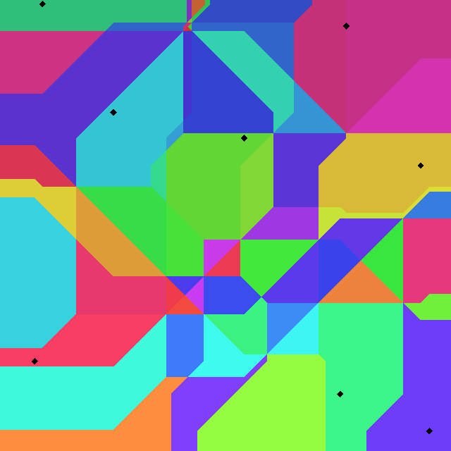
This post is about a generalization of Voronoi diagram that I played around with. It’s probably not that useful but it’s a little fun math with an absolute ton of colorful diagrams.

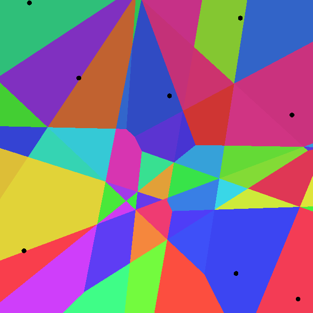
It occurred to me a while ago that there was a generalization of Voronoi diagrams that maybe could be useful to something I was working on. As you know, a Voronoi diagram divides the plane into regions based on a set of points. Given the points, p₀, p₁, …, p_n, the region corresponding to p_i is the set of points that are closer to p_i than any of the other p_j. Here is an example of a run-of-the mill, standard, plain vanilla, Voronoi diagram:

This diagram determines which points are closer using normal, cartesian, distance but Voronoi diagrams also make sense for other kinds of distance, for instance Manhattan distance:

The generalization that occurred to me was: if a region in a plain Voronoi diagram is defined by the one point it is closest to, what if you defined a diagram where regions are based on the two closest points? That is, for each pair of points, p_i and p_j, there would be a region made up of points where the closest point is p_i and the second-closest is p_j. What would that look like, I wondered. I searched around and it’s definitely a thing, it’s called a higher-order Voronoi diagram, but I couldn’t find any actual diagrams.

There may be some established terminology around this but I ended up using my own names: I would call what I just described a Voronoi² diagram, and a plain one would be a Voronoi¹. (From here on I’ll call the region around p_i in the Voronoi¹ diagram V(p_i), and the region around p_i and p_j in the Voronoi² diagram I’ll call V(p_i, p_j)).

You can kind of guess just from the definition that a Voronoi² would look similar to the corresponding Voronoi¹ just more subdivided. For any given p_i, the point’s region in the Voronoi¹ diagram, V(p_i), is the set of point closest to p_i. Well for any point in that set they will have some other point p_j as their second-closest, and so if you take the union over all p_j of V(p_i, p_j) that gives you V(p_i). So the regions in a Voronoi² diagram are basically fragments of regions of the Voronoi¹.

Below is the same diagram as before, for comparison, and the Voronoi² diagram.

• 

• 

As you can see, that is exactly what the Voronoi² diagram looks like: each Voronoi¹ region has been subdivided into sub-regions, one for each of its neighboring points. You can do the same thing for the Manhattan diagrams,

• 

• 

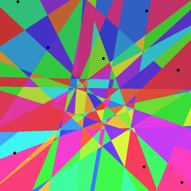
Now we’ve defined Voronoi¹ and Voronoi² but why stop there when we could keep going and define Voronoi³. This would be, you’ve probably already guessed it, a diagram with a region for each choice of p_i, p_j, and p_k, that is made up of the points that have p_i as their closest point, p_j as their second-closest, and p_k as their third-closest. Let’s call such a region V(p_i, p_j, p_k). As I’m sure you’ve already guessed the Voronoi³ regions are further subdivisions of the Voronoi² regions:

• 

• 

• 

And the Manhattan version,

• 

• 

• 

The images are becoming smaller but you can click them to see larger versions.

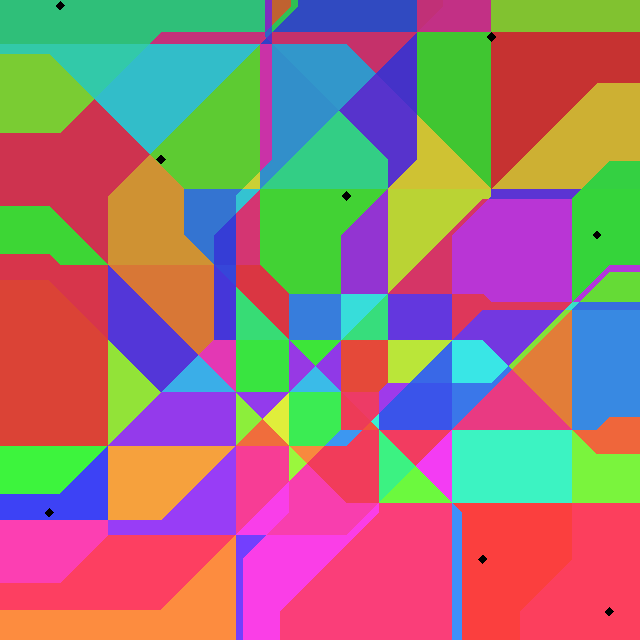
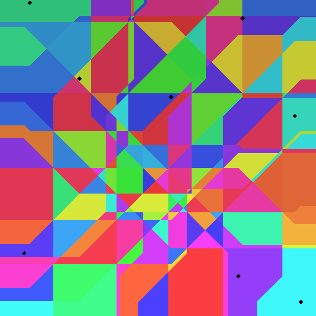
From here you can just keep going: Voronoi⁴, Voronoi⁵, Voronoi⁶, and so on and so on. Which of course I did, what did you expect? Here are Voronoi¹-Voronoi⁸ with cartesian distance,

• 

• 

• 

• 

• 

• 

• 

• 

and the same with Manhattan distance

• 

• 

• 

• 

• 

• 

• 

• 

Except… I lied before when I said you could just keep going. In this example there are 8 points so the Voronoiⁿ diagrams are only well-defined for n up to 8 – that’s why there’s 8 diagrams above. And indeed if you look closely diagram 7 and 8 are actually the same – because once you’ve picked 7 points there is no choice for the last point, there is only the 8th left, so the diagrams end up looking exactly the same.

So is that it – is that all the colorful diagrams we get? Well, there is just one last tweak we can make to get a different kind of diagram.

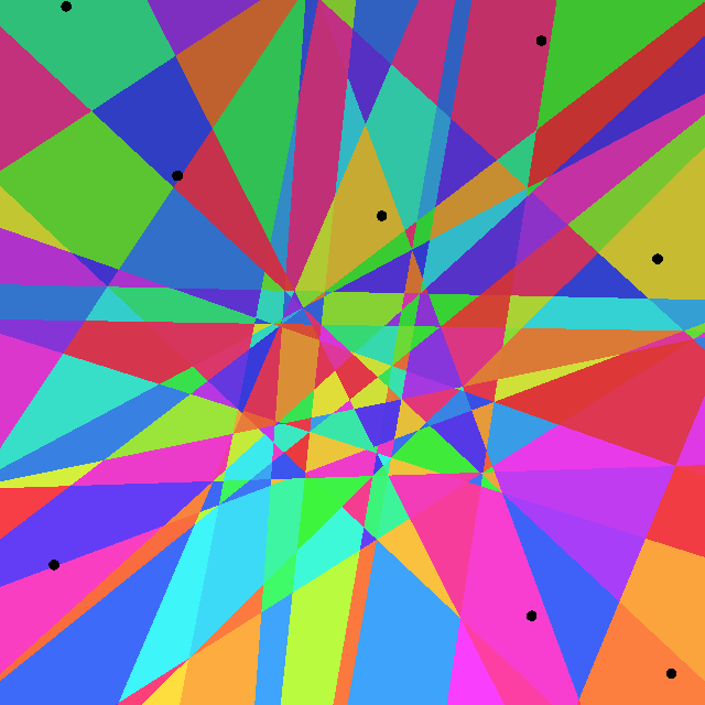
The thing is, in the definition of Voronoi² we said that V(p_i, p_j) was the points where p_i is the closest point and p_j is the second-closest. That is, the order of p_i and p_j is significant. An alternative definition we could use would be one where we don’t consider the order, where the region doesn’t care whether it’s p_i closest and p_j second-closest, or p_j closest and p_i second-closest. I’ll call this V_u(p_i, p_j) (the u is for unordered).

You’ll notice right away that by this definition V_u(p_i, p_j)=V_u(p_j, p_i) so there’s a lot fewer regions. Here’s an example of a Voronoi_u¹ (which is the same as the Voronoi¹) and Voronoi_u² diagram,

• 

• 

With these unordered diagrams it can be a little trickier to figure out which two points a region actually corresponds to, especially in cases where the points in question are far away from the region. The trick you can use in this case is that for a given region is in the Voronoi_u², if you look at the same place in the Voronoi¹ there will be a dividing line that goes across where the region is in the Voronoi_u², from one corner of the region to another. The two points on either side of the Voronoi¹ will be the one the region corresponds to.

The same things works, as always, with Manhattan distance:

• 

• 

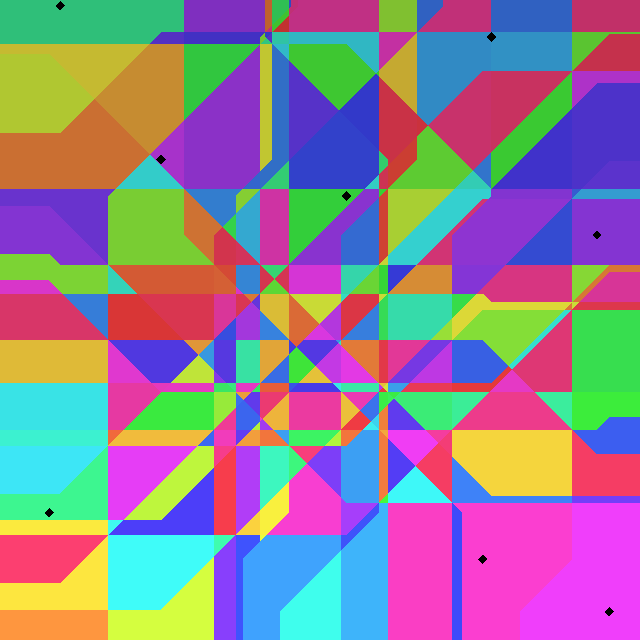
An interesting thing happens if we plot all the Voronoi_uⁿ all the way up to 8:

• 

• 

• 

• 

• 

• 

• 

• 

The number of regions stays about the same and when we get to Voronoi_u⁷ and Voronoi_u⁸ they actually become simpler. This is because at that point the set of points for a given region includes almost all the points so the determining factor becomes which are the few points that aren’t in the set – and at 7 and 8 there’s 1 and 0 left respectively. So whereas Voronoi⁸ was useless because it’s the same as Voronoi⁷, here it’s useless because there’s only one region that contains all the points.

Is this construction at all useful? I’m not sure, I imagine it could be but I don’t have any particular use for them myself. Really I was just curious what it would look like.

I’ll leave you with a last set of diagrams, Voronoi_u¹ to Voronoi_u⁸ for Manhattan distance.

• 

• 

• 

• 

• 

• 

• 

• 

I haven’t written much about it on this blog but the project I’ve been working on full time for the last two years is a new kind of terminal, chorus. Current terminals are a relic of the past and chorus is my take on a modern replacement.

I’ve created a blog specifically about chorus, the chorus console blog. There I’ll be writing about the approach I’m taking and my thoughts about what terminals are and where they should be moving. The title of this post itself hints at where I see them evolving. But you can read more about that in the introductory post.

I have this problem where I need to try something a number of times, maybe 64 times, and each time with a different small seed, say a value between 0 and 1024. I’d like the seeds to be reasonably scrambled and I don’t want to see the same one more than once. I also need the same order every time, that’s what I mean by pre-scrambling – the scrambling isn’t dynamic, it’s hardcoded. How do I do this in a simple way without resorting to say just hard coding a list of numbers?

What I’d really like to do is use something like a random number generator but with pre-determined set parameters that I know will generate the numbers I want. The xorshift generator seems like a good candidate because it’s really simple but the quality is decent. It requires 4 parameters, x, y, z, and w, and then you can generate a sequence of values in the following way, where limit is the size of the set you want to generate:

t = x ^ (x << 11) & 0xFFFFFFFF
x = y
y = z
z = w
w = (w ^ (w >> 19) ^ t ^ (t >> 8)) & 0xFFFFFFFF
return w % limit

This is what I’d like to use — I just need some parameters. And it turns out that there are parameters that will make it behave like I want. Here’s an example,

0x31f12daf 0x6dd97342 0xda4daacd 0x41235c71: 85/256 85 (33.2% 1x)

This means: with these parameters x y z w and a limit of 256 you get 85 different values (that’s the 85 in “85/256”) if you execute the xorshift code 85 times (that’s the second 85), which means that you’re covering 33.2% of the possible values and executing the loop 1x per unique generated value. Here are some seeds for different limits that are powers of 2, that generate a pretty big set of unique values,

0x2735e8f4 0x9fcb0c3e 0xd0c18064 0x0f6b0093: 26/32 26 (81.2% 1x)
0x1ff079d6 0x54248059 0xc968e911 0x38c15c75: 39/64 39 (60.9% 1x)
0xf8efc789 0x88a40b37 0x86f01aa6 0x15384f52: 59/128 59 (46.1% 1x)
0x31f12daf 0x6dd97342 0xda4daacd 0x41235c71: 85/256 85 (33.2% 1x)
0xfd8193d0 0xc8b69d8f 0xa42b9d1c 0x7e69d727: 133/512 133 (26% 1x)
0x4617b049 0xf7a49270 0xa88b568c 0x32dff77c: 174/1024 174 (17% 1x)

As an example of how to use one of these, here’s how you’d use the first line, the one that generates values with a limit of 32, in python:

def generate():
  x = 0x2735e8f4
  y = 0x9fcb0c3e
  z = 0xd0c18064
  w = 0x0f6b0093
  for i in range(0, 26):
    t = (x ^ (x << 11)) & 0xFFFFFFFF
    x = y
    y = z
    z = w
    w = (w ^ (w >> 19) ^ t ^ (t >> 8)) & 0xFFFFFFFF
    yield w % 32

print list(generate())

This prints

[2, 18, 9, 30, 12, 0, 19, 17, 7, 5, 14, 16, 6, 24, 15, 4, 3,
31, 10, 29, 8, 23, 11, 22, 1, 26]

which, and you can check if you want, are 26 different values between 0 and 32.

If you can tolerate some duplicates you can get better coverage. If you can only tolerate a few, say about one duplicate in 16 values, you can get,

0xf852d2f8 0xaf137287 0x6a0d4795 0x326c8a41: 28/32 29 (87.5% 1x)
0xa8683488 0x361c1383 0xbc95298a 0xe4c57646: 46/64 49 (71.9% 1.1x)
0xca30a753 0x317aa350 0x1bc8bee2 0xce4830bf: 79/128 87 (61.7% 1.1x)
0xe079cdb3 0x7cb29574 0x45eebac8 0xeb8dcefc: 132/256 147 (51.6% 1.1x)
0xf41e4441 0x3345d823 0x608ff840 0x554f5cdd: 238/512 269 (46.5% 1.1x)
0x201ceef2 0x7f49ce17 0x0bd10615 0x139bfa7b: 423/1024 485 (41.3% 1.1x)

So for example in the 256 case, if you generate 147 values with the given seed you’ll hit 132 different values between 0 and 256, and the rest will be duplicates. That’s a lot better coverage than the 85 you could hit if you didn’t allow them.

If you can tolerate even more duplicates, say you don’t mind hitting roughly one on average per unique value, you can get close to full coverage

0xa9bb0026 0xe0178ff2 0x443fd052 0x9fe0d459: 32/32 41 (100% 1.3x)
0x4c19f4c7 0x1d253873 0x5c1f6f17 0x812944fc: 64/64 106 (100% 1.7x)
0x854fbffe 0x5aa965d5 0x06ff8c3e 0xd5057351: 127/128 252 (99.2% 2x)
0xeb03a458 0x26ae990e 0x6227aaee 0x192b3cb7: 242/256 496 (94.5% 2x)
0x97bbc402 0x20470416 0x09ce179b 0xbf276b7d: 469/512 980 (91.6% 2.1x)
0x6d36254c 0x19c5f46a 0x1614da1a 0xcfadbfc8: 915/1024 1939 (89.4% 2.1x)

As an example, running the same python code from above but now with parameters from this set you get,

[19, 27, 10, 12, 18, 16, 13, 15, 24, 4, 23, 11, 28, 30, 26,
19, 24, 1, 12, 15, 29, 2, 19, 8, 9, 20, 6, 5, 17, 3, 14, 31,
22, 25, 18, 27, 8, 20, 0, 7, 21]

In this list of length 41 all numbers between 0 and 31 occur, but 8, 12, 15, 18, 20, 24, and 27 are there twice and 19 is there three times.

Finally, if you don’t care how many times you try as long as you generate all the numbers that’s possible too. At this point you probably want to keep track of which value you’ve seen, maybe with a bit vector, and just filter the raw values you generate.

0xa9bb0026 0xe0178ff2 0x443fd052 0x9fe0d459: 32/32 41 (100% 1.3x)
0x4c19f4c7 0x1d253873 0x5c1f6f17 0x812944fc: 64/64 106 (100% 1.7x)
0xf3bd4634 0xb1442411 0xd536236f 0x3beae2fb: 128/128 291 (100% 2.3x)
0x1c608f31 0x34e54bbd 0xa799c7a8 0x78af6664: 256/256 729 (100% 2.8x)
0x10bace53 0x88bc0781 0xd815fe20 0xc77bcbec: 512/512 1786 (100% 3.5x)
0xb6c93670 0xb89f9de6 0x3ba3713c 0x78bcabc7: 1024/1024 4341 (100% 4.2x)

If you look closely you’ll notice that the parameters are the same as before for some limits, that’s because we already had perfect coverage before so there’s nothing to improve. And as the set grows you can see that the number of times you have to try grows, so at 1024 you need to loop 4341 times before you’ve seen all values. And note also that the duplicates aren’t evenly distributed, the further you get the more work you have to do to get a value you haven’t seen before.

Of limited use I guess but if this is the kind of thing you need, pretty convenient. I’ve dumped the code I used to generate these in a gist.

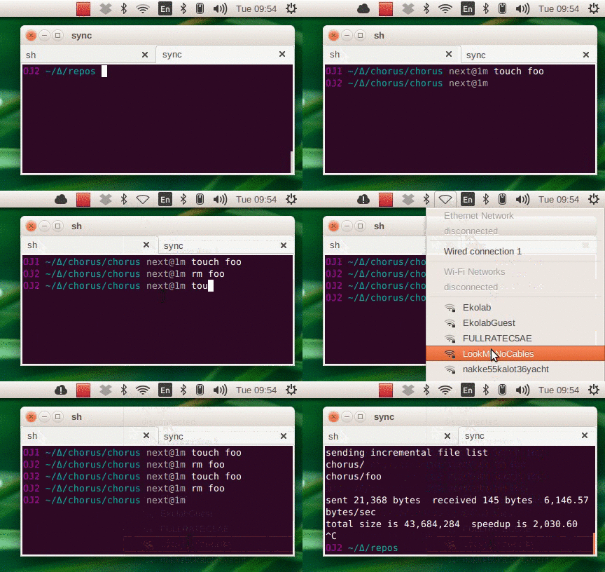
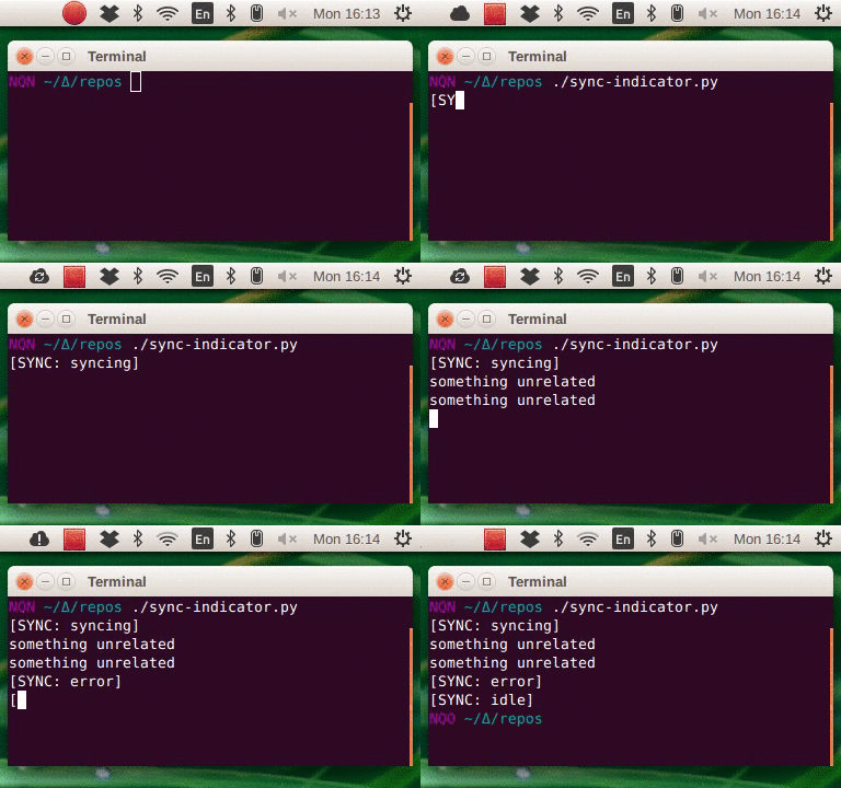
This post is about interacting with the graphical desktop environment from a shell script. Specifically: say you have a long-running bash script and you’d like to keep an eye on it through a unity app indicator. How do you make that work in an appropriately unix-y way? (If you’re not sure what I mean see the animation below).

Background. Over the weekend I finally changed from NFS to rsync for keeping my source code in sync across machines. Much better if my network connection is unreliable and fewer moving parts. After I was done with the basics though I thought: I really need to be able to keep an eye on how syncing is going. It’s just the worst to spend ages unsuccessfully trying to reproduce an issue on a virtual machine only to realize that it’s because the code I’m running isn’t being properly synced when I edit files on my laptop.

Here’s what I had in mind: when I run the code change monitor shell script I want to get an app indicator in the top bar that changes state when a sync is going on, so I can see that syncing actually happening and whether it’s slow. And I want it to show if there are any errors. This, in other words

The syncing logic itself is straightforward: one component uses inotifywait to wait for files to change (watchdog.sh), then calls out to a script that does the actual sync (do-rsync.sh).

How to show the indicator though? There is no command-line api for this kind of thing and I wasn’t sure what it would look like if there was. Also, the existing code was properly unix-y and I wanted it to stay that way. One component knows how to wait for changes but knows nothing about rsync; the rsync part knows how to do a single sync but doesn’t care when or why it is being called. They only meet at the top level,

watchdog.sh --root . ./do-rsync.sh

What I ended up with was a python script, sync-indicator.py, that was responsible for just the indicator. When it starts it creates the indicator and then waits around, reading input from stdin. When it sees a command in the output it recognizes, say [SYNC: syncing], it consumes that line and changes the state of the indicator. Anything that doesn’t match is just passes straight through to stdout. Here’s what it looks like,

This way the indicator logic doesn’t need to know about the watching or rsyncing, and those parts don’t need to know about the indicator. All you need to do is change the toplevel command that puts it all together to,

watchdog.sh --root . ./do-sync-and-indicate.sh | ./sync-indicator.py

where do-sync-and-indicate.sh is a trivial wrapper around do-sync.sh that looks like this,

#!/bin/bash

echo "[SYNC: syncing]"
if ./do-sync.sh; then
  echo "[SYNC: idle]"
else
  echo "[SYNC: error]"
fi

You can even replace this with a generic command that takes another command as an argument and all it does is call that command surrounded with appropriate SYNC messages.

Pretty clean and unix-y I think, independent components and so on.  The python indicator script itself, sync-indicator.py, is straightforward, only 60ish lines with comments.

The ease of supporting this makes me wonder though. Why aren’t long-running commands better at interacting with the desktop?

I’ve been reading Learn You a Haskell and got stuck on a tiny point at the beginning, in the section about ranges: you can’t have a range with more than one step value. This post is about what it might mean to allow multiple steps and how Charles Babbage might have had an opinion on this particular aspect of haskell’s design.

Here’s the whole paragraph from Learn You a Haskell,

To make a list containing all the natural numbers from 1 to 20, you just write [1..20]. [… snip …] Ranges are cool because you can also specify a step. What if we want all even numbers between 1 and 20? Or every third number between 1 and 20?

ghci> [2,4..20]
[2,4,6,8,10,12,14,16,18,20]
ghci> [3,6..20]
[3,6,9,12,15,18]

It’s simply a matter of separating the first two elements with a comma and then specifying what the upper limit is. While pretty smart, ranges with steps aren’t as smart as some people expect them to be. You can’t do [1,2,4,8,16..100] and expect to get all the powers of 2. Firstly because you can only specify one step. And secondly because some sequences that aren’t arithmetic are ambiguous if given only by a few of their first terms.

The bold highlight is mine. This makes sense – how can the language guess that what you have in mind when you write [1, 2, 4, 8, 16..] is the powers of 2?

On the other hand though, just as a fun exercise, if you were to allow multiple step values how would you define them? Even though this is a highly specialized and modern language design question I know Charles Babbage would have understood it and I suspect he would have had an opinion.

A while ago I wrote a post about Babbage’s difference engine. The difference engine is basically an adder that calculates successive values of a polynomial by doing simple addition, using a technique called divided differences. This is described in full detail in that post but here’s a summary. Take a sequence of values of values of a polynomial, for instance the first four squares,

You can then calculate the next values using just addition by calculating the differences between the initial values. To get the differences for a sequence you subtract each pair of values,

Do it once and you get the first differences. Do the same thing to the first differences and you get the second differences,

Do the same thing to the second differences and you get the third differences,

In this case there’s just one and it’s 0 so we can ignore it. Once you have all the differences you can calculate the next value of the polynomial by adding them together from right to left,

There it is, 16, the next value in the sequence. At this point we can just keep going,

This technique works for any polynomial. The difference engine was given its name because it is a mechanical implementation of it.

Already you may suspect how this can be relevant to ranges in haskell. You can generalize ranges to n step values by using divided differences on the step values to generate the rest of the sequence. With two step values the result of this is a linear sequence, as you would expect (polyEnumFrom is my name for the generalized range function),

ghci> polyEnumFrom [0, 1]
[0, 1, 2, 3, 4, 5, 6, ...]
ghci> polyEnumFrom [4, 6]
[4, 6, 8, 10, 12, 14, 16, ...]
ghci> polyEnumFrom [10, 9]
[10, 9, 8, 7, 6, 5, 6, ...]


Give it three elements, for instance the squares from before, and the result is a second-order polynomial,

ghci> polyEnumFrom [0, 1, 4]
[0, 1, 4, 9, 16, 25, 36, ...]

Similarly with the cubes,

ghci> polyEnumFrom [0, 1, 8, 27]
[0, 1, 8, 27, 64, 125, 216, ...]

There is nothing magical going on here to recognize the squares or cubes here, it’s a completely mechanical process that uses subtraction to get the differences and addition to then continue the sequence past the step values. It won’t give you the squares though, only polynomials. If you try you get

ghci> polyEnumFrom [1, 2, 4, 8, 16]
[1, 2, 4, 8, 16, 31, 57, ...]

For any list of 3 step values there is exactly one polynomial of order 2 or less that yields those values; an order-2 polynomial has 3 free variables so there’s no room for more than one solution. The result of a 3-step range is the sequence of values produced by that order-2 polynomial. In general, the result of a multi-step range with n steps is the sequence of values generated by the unique polynomial of order at most n-1 whose first n values are the steps. Conveniently, if the steps are integers the polynomial is guaranteed to only produce integers.

Babbage built the difference engine because it was really important then be able to produce tables of function values by calculating successive values of polynomials. I think he would have appreciated the power of a language where you can condense the work of generating an approximate table of sine values into a single line,

take 10 (polyEnumFrom [0, 0.0002909, 0.0005818, 0.0008727])

which yields,

0.0000000
0.0002909
0.0005818
0.0008727
0.0011636
0.0014545
0.0017454
...

(The four values given to polyEnumFrom are the first four sine values from the table.) Of course, Babbage did lose interest in the difference engine himself and preferred to work on the more general analytical engine. If he did see haskell he would probably quickly lose interest in ranges and move on to more general advanced features. But I digress.

Is a shorthand for sequences of polynomial values actually a useful feature in a language? I doubt it. But I like the idea that a corner of a modern language  intersects with Babbage and the difference engine. Maybe it would make sense as a little easter-egg tribute to Babbage, a difference engine hiding behind a familiar language construct. I quite like the idea of that.

If you want to play around with it I’ve put an implementation in a gist. For something that might seem fairly complex the implementation is simple – polyEnumFrom and its helpers is just 13 lines. Haskell is an elegant language.

This is the third post in a series about z-quads, a spatial coordinate system. The first one was about the basic construction, the second about how to determine which quads contain each other. This one is about conversions: how to convert positions to quads and back.

First, a quick reminder. A quad is a square(-ish) area on the surface of the earth. Most of the time we’ll use the unit square instead of the earth because it makes things simpler and you can go back and forth between lat/longs and unit coordinates just by scaling the value up and down. (There’s a section at the end about that.)

So, when I’m talking about encoding a point as a quad, what I mean more specifically is: given a point on the unit square (x, y) and a zoom level z, find the quad at zoom level z that contains the point. As it turns out, the zoom level doesn’t really matter so we’ll always find the most precise quad for a given point. If you need a different zoom level you can just have a step at the end that gets the precise quad’s ancestor at whatever level you want.

Precision

So far we’ve focused on quads as an abstract mathematical concept and there’s been no reason to limit how far down you can zoom. In practice though you’ll want to store quads in integers of finite size, typically 32-bit or 64-bit. That limits the precision.

It turns out that you can fit 15 zoom levels into 32 bits and 31 into 64. At zoom level 15 the size of a quad is around 1.5 km². At zoom level 31 it’s around 3 cm². So yeah, you typically don’t need more than 31 levels. A third case is if you want to store your quad as a double – JavaScript, I’m looking at you here. A double can hold all integers up to 53 bits, after which some can’t be represented. That corresponds to 26 zoom levels which is also plenty precise for most uses.

Encoding points

Okay, now we’re ready to look at encoding. What we’ll do is take a unit point (x, y) and find the level 31 quad that contains it. Since we’ve fixed the zoom level we’ll immediately switch to talking about the scalar rather than the quad. That makes everything simpler because within one level we’re dealing with a normal z-order curve and conversion to and from those are well understood.

The diagram on the right illustrates something we’ve seen before: that scalars are numbered such that the children at each level are contiguous. In this example, the first two green bits say which of the four 2×2 divisions we’re in. The next two say which 1×1 subdivision of that we’re in. It’s useful to think of this the same way as the order of significance within a normal integer: the further to the left a pair of bits is in a scalar the more significant it is in determining where the scalar is.

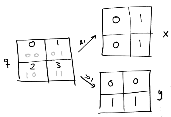
Now things will have to get really bit-fiddly for a moment. Let’s look at just a single 2×2 division. Each subdivision can be identified with an (x, y) coordinate where each ordinate is either 0 or 1, or alternatively with a scalar from 0 to 3. The way the scalars are numbered it happens that the least significant scalar bit gives you the x-coordinate and the most significant one gives you y:

(This is by design by the way, it’s why the z-shape for scalars is convenient). This means that given point x and y, each 0 or 1, you get the scalar they correspond to by doing

x + 2 y

What’s neat about that is that because of the way pairs of bits in the scalar increase in significance from right to left matches the significance of bits in an integer, you can do this for each bit of x and y at the same time, in parallel. To illustrate how this works I’ll take an example.

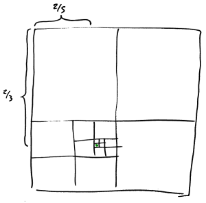
Let’s start with the point (2/5, 2/3) and find the level 5 scalar that contains it. First we’ll multiply both values by 3² (=2⁵) and round the result to an integer,

x = (2/5) × 32 ≈ 12 = 01100b
y = (2/3) × 32 ≈ 21 = 10101b

Now we’ll perform x + 2 y for each bit in parallel like so,

Looks bizarre right, but it does work. We spread out the bits from each input coordinate so they can be matched up pairwise and then add them together. The result is the scalar we’re looking for because the order of significance of the bit-pairs in the scalar match the significance of the individual bits in each of the inputs.

Now, how can you tell that the result, scalar 626 on zoom level 5, is the right answer? This diagram suggests that it’s about right:

The bit-pairs in the scalar are [2, 1, 3, 0, 2]  so we first divide and take subdivision 2, then divide that and take 1, then divide that, and so on. Ultimately we end up at the green dot. In this case the last step would be to add the appropriate bias, b₅, to get a proper quad and then we’re all done.

Because this conversion handles all the levels in parallel there’s little benefit to converting to a higher zoom level than the most precise, typically 31. If you want level 5 do the conversion to level 31 and then get the 26th ancestor of the result.

Most of the work in performing a conversion is spreading out the scaled 31-bit integer coordinates. One way to spread the bits is using parallel prefix which takes log₂ n steps for an n-bit word,

  00000000abcdefgh
→ 0000abcd0000efgh
→ 00ab00cd00ef00gh
→ 0a0b0c0d0e0f0g0h

That’s just one way to do it, there are others.

Decoding quads

The operation above gets you into quad-land and obviously you’ll want to be able to get out again. This turns out to just be a matter of running the encoding algorithm backwards. The main difference is that here we’ll stay on whatever zoom level the quad’s on instead of always going to level 31.

Given a quad q this is how you’d decode it:

1. Subtract the bias to get the quad’s scalar.
2. Mask out all the even-index bits to get the spread x value and the odd-index bits to get the spread y value. Shift the y value right by 1.
3. Pack the spread-x and –y values back together to get a z_q-bit integer value for each. Packing can be similarly to spreading but in reverse.
4. Floating-point divide the integer values by 2^z_q. You now have your (x, y) coordinates between 0 and 1.

A quad is an area but the result here is a point, the top left corner of the quad. This is often what you’re interested in, for instance if you’re calculating is the full area of the quad. There you can just add the width and height of the quad (which are both 2^–z_q) to get the other corners. Alternatively you might be interested in the center of the quad instead. To get you can modify the last step of the algorithm to do,

Apply (2 v + 1) / 2^z_q+1 as a floating-point operation to each of the integer coordinates.

This is just a circuitous way to add 0.5 to v before dividing by 2^z_q but this way we can keep the value integer until the final division. If you want to minimize the loss of precision when round-tripping a point through a quad you should use the center since it’s the point with the smallest maximum distance to the points that belong to that quad.

So, now we can convert floating-point coordinates to quads and back again with ease. Well, relative ease. In the last part I’ll talk briefly about something I’ve been hand-waving until now: converting from lat/long to the unit square and back.

Latitude and longitude

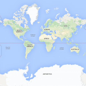
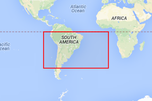
When you encounter a lat/long it is typically expressed using the WGS 84 standard. The latitude, a value between -90 and 90, gives you the north-south position. The longitude, a value between -180 and 180, gives you east-west.

A typical world map will look something like the one on the right here with America to the left and Asia to the right. The top left corner, northwest of North America, is lat 90 and long -180. The bottom right, south of New Zealand, has lat -90 and long 180. You could convert those ranges to an (x, y) on the unit square in any number of ways but the way I’ve been doing it follows the z-order curve the same way I’ve been using in this post: North America is in division 0, Asia in division 1, South America in division 2, and Australia in division 3. The conversion that gives you that is,

x = (180 + long) / 360
y = (90 – lat) / 180

This puts (0, 0) in the top left corner and (1, 1) in the bottom right and assigns the quads in that z-shaped pattern.

There’s a lot to be said about map projections at this point. I limit myself to saying that while it’s convenient that there’s a simple mapping between the space most commonly used for geographic coordinates and the space of quads, the Mercator projection really is a wasteful way to map a sphere onto a square. For instance, a full third of the space of quads is spent covering the Southern Ocean and Antarctica even though they take up much less than a third of the surface of the globe. I’d be interested in any alternative mappings that make more proportional use of the space of quads.

Okay, so now there’s a way to convert between WGS 84 and quads. I suspect there’s a lot more you can do with z-quads but this, together with the operations from the two previous posts, what I needed for my application so we’re at to the end of my series of posts about them. Well, except for one final thing: string representation. I’ve always been unhappy with how unmemorable geographic positions are so I made up a conversion from quads to sort-of memorable strings which I’ll describe in the last post.

In the meantime I made a little toy site that allows you to convert between positions and quads at a given zoom level. Here is an example,

This is quad 167159423 at zoom level 14 which covers, as always, Århus. The URL is

http://zquad.p5r.org?latlng=56.1676,10.2062&zoom=14

which kind of explains itself. You can also do

http://zquad.p5r.org?address=San+Francisco&zoom=14

Finally to see where a particular quad is try

http://zquad.p5r.org?quad=15386

If you want to explore the space of quads you can play around with the parameters yourself.

This post is about a spatial coordinate system I’ve been playing around with, z-quads. Unlike most commonly used coordinate systems a z-quad doesn’t represent a point but a square with an area.

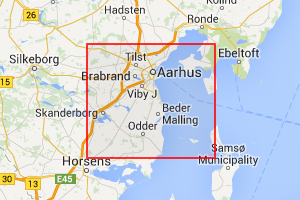
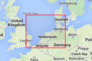
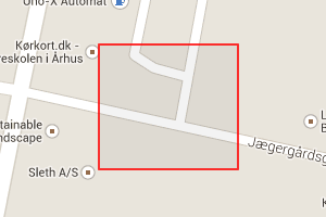
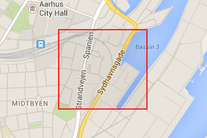
To the right are some examples of quads of increasing accuracy, gradually zooming in on Århus. (The quads are the red rectangles). The first one that covers northern Germany, some of England, and half of Denmark, is quad 637 which has zoom level 5. The one that covers all of Århus is 163241 which has zoom level 9. Going further down to zoom level 15 is 668638046 which covers part of the center of Århus, and finally at zoom level 19 is 171171340006 which covers just a couple of houses.

This should give a rough sense of how the system works. A quad is an integer, typically 64 bits, which represents some square area on the earth. Each quad has a zoom level associated with it and higher numbers have higher zoom levels. There’s a lot more to it than that but that’s the core of it.

Below I’ll describe how z-quads are constructed, which is pretty straightforward. Then I’ll look at how to operate on them: how to convert to and from them, zoom in and out, that kind of thing.

Divide, divide, divide some more

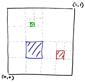
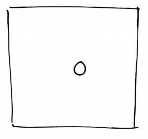
For a hobby project I’m working on I needed to represent a large set of geographic coordinates. They happen to represent positions of bus and train stops but that’s not super important. To the right is a diagram that illustrates what I had in mind when I started playing around with this. What I wanted really was a way to divide the world evenly into squares of different sizes that I could divide my positions into. (For simplicity I’ve scaled the world down to a 1×1 unit square). Each of the three colored squares here should have some unique integer id. When I say “divide the world evenly” I mean that they’re not arbitrary squares, they’re on the grid you get if you divide the whole square into in four equal parts, then divide each of those into four as well, and so on and so on.

It seemed intuitively reasonable that you’d want the entire space to be represented by 0.

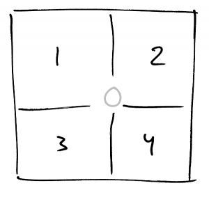
This is zoom level 0. Zooming down one level, you might divide 0 into four parts and call them 1-4,

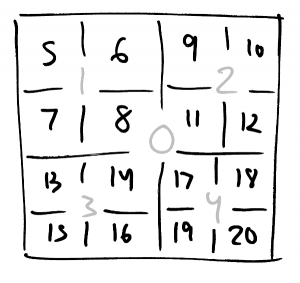
This is zoom level 1. Then you can keep going and do the same again to get zoom level 2,

At each new zoom level you add 4 times as many new quads as you had on the previous level so where level 2 has 16, level 3 will have 64 and level 4 will have 256.

This is how z-quads are constructed. Pretty simple right? Already, by the way, we know the id of the blue square from the beginning because it’s there at zoom level 2: it’s quad 14. And just as a reminder, at this point we’re playing around on the unit square but it’s just a matter of scaling the values back up to get coordinates on the earth. Here’s 14 again, scaled back up:

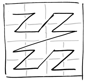
One thing you may notice if you look closely at how the quads at zoom level 2 are numbered is that they look of out of sequence. You might expect them to be numbered 5-8 on the top row, 9-12 on the next, and so on. Instead they’re numbered in zig-zag, like this:

So they zig-zag within each of the four parts of the big square, and also when going between the four parts. That’s because it turns out to be really convenient when you divide a quad to have all the quads in the subdivisions be contiguous. So the children of 1 are 5-8, of 2 are 9-12, and so on. We’ll end up relying on that constantly later on. (The numbering within each level it known as a Z-order or Moreton order curve).

Okay, so now I’ve postulated way to divide the unit square, by which I mean the surface of the earth, into regular parts. The next step is to figure out how to operate on them which is where it’ll become clear why this number is is particularly appealing.

Zoom bias

Given a quad there are many operations that you might conceivably want to perform. You might want to know which quad is its parent (that is, the quad that contains it at the zoom level above) or the parent’s parent, etc. Given two quads you might want to know whether one contains the other. Or you might want to find the most specific quad that contains both of them.

The first thing we’ll look at is how to get the parent of a quad. To explain that I need to introduce two contepts, zoom bias and a quad’s scalar. The zoom levels we’ve seen so far (and a few more) and the values of their quads are

• Zoom 0: 0
• Zoom 1: 1-4
• Zoom 2: 5-20
• Zoom 3: 21-84
• Zoom 4: 85-341

In general, at level z you have 4^z quads, so at level 2 you have 4²=16, the first one being 5. At level 3 you have 4³=64, the first one being 21, and so on.

The value of the first quad for a given zoom level turns out to appear again and again when doing operations so I’ll give that a name: the zoom bias. When I talk about the zoom-3 bias, which I’ll typically write as b₃, what I’m referring to is 21 since that is the value of the first quad at zoom level 3.

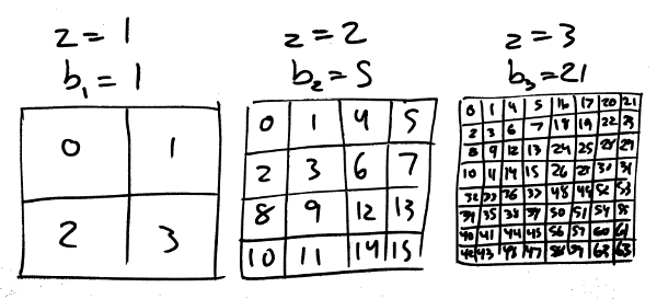
The scalar of a quad is its value minus the bias of its zoom level. Here are the biases and scalars for zoom levels 1 to 3:

Parents and children

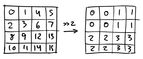
Now we’re ready to look at how you get a quad’s parent. As mentioned, quads are numbered such that the subquads of each parent are contiguous. That obviously also holds for the scalars. That means that if you divide the scalar value by 4, the number of children in each parent, this happens:

You get the scalar of the parent. So given a quad q at zoom level z, the parent quad can be computed as

parent(q) = ((q – b_z) / 4) + b_z-1

Unbias the quad to get the scalar, divide it by 4 to get the parent’s scalar, then add the parent’s zoom level bias to get back a quad. And in fact this can be simplified if you use the fact that the zoom biases are related like this,

b_z+1 = 4b_z + 1

I’ll justify this in a moment but for now you can just take it as a given. If you plug this in and simplify you get that

parent(q) = (q – 1) / 4

(By the way, except when stated explicitly all values are integers so division implicitly rounds down). What’s neat about the simplified version is that b_z no longer appears so you can apply this without explicitly knowing the zoom level. It’s pretty easy to calculate the zoom level for a quad, I’ll go over that in a bit, but it’s even easier if you don’t have to.

How about going the other way? Given a quad, finding the value of one of its children? That’s the same procedure just going the other way: unbias the parent, multiply by 4, add the child’s index (a value from 0 to 3), rebias:

child(q, i) = 4(q – b_z) + i + b_z+1

Again this can be simplified by using the relation between the zoom biases to

child(q, i) = 4q + i + 1

If instead of the child’s index (from 0 to 3) you use its quad value (from 1 to 4) it becomes even simpler,

child(q, i) = 4q + i

This is part of why they’re called z-quads: it’s from all the z-words. The numbering zig-zags and it’s easy to zoom in and out, that is, get between a quad and its parent and children. (If, by the way, you’ve ever used a d-ary heap you may have noticed that this is the same operation used to get the child node in a 4-ary heap).

Since you can calculate the value of a child quad given its parent it also means that you can calculate the value of a quad one zoom level at a time, starting from 0. For instance, in the original example with the colored squares the blue square was child 2 of child 3 of 0. That means the value is

child(child(0, 3), 2) = 4 (4 0 + 3) + 2 = 4 3 + 2 = 12 + 2 = 14

Which we already knew from before of course. This isn’t how you would typically convert between positions and quads in a program, there’s a smarter way to do that, but I’ve found it useful for pen-and-paper calculations.

Ancestors and descendants

Now we know how to go between a quad and its parent and children we can generalize it to going several steps. When going multiple steps, instead of talking about parents and children we’ll talk about ancestors and descendants. An ancestor of a quad is its parent or one of the parent’s ancestors. A descendant of a quad is one of its children or one of the children’s descendants.

It turns out that just as there’s a simple formula for getting a quad’s parent there is one for getting any of its ancestors:

ancestor(q, n) = (q – b_n) / 4ⁿ

Given a quad this gives you the ancestor n steps above it. The special case where n is 1 is the parent function from before, b₁ being 1. Even though it might not seem sensible now it’s worth noting for later that this is also well-defined for n=0 where the result is q. So a quad is its own 0th ancestor.

It’s easy to prove that the ancestor function is correct inductively by using a second relation that holds between the b_zs:

b_z+1 = 4^z + b_z

I won’t do the proof here but maybe we should take a short break and talk about why these relations between the biases hold. The bias at a zoom level is the index of the first quad at that level. At level 0 there is 1 (=4⁰) quad so b₁, the next available index, is 1. At level 1 there are 4 (= 4¹) which start from 1 so the next bias is

b₂ = 4⁰ + 4¹ = b₁ + 4¹ = 5

If we keep going, the next level adds 16 (= 42) quads in addition to the 5 we already have which makes the next bias

b₃ = 4⁰ + 4¹ + 4² = b₂ + 4² = 21

You can see how each bias is a sum of successive powers of 4 which gives you the relation I just mentioned above, that to get the next bias you just add the next power of 4 to the previous bias.

b₃ = b₂ + 4²

It also gives us the other relation from earlier,

b₃ = 4⁰ + 4¹ + 4² = 4⁰ + 4(4⁰ + 4¹) = 4 b₂ + 1

Okay so back to ancestors and descendants. As with ancestors you can also get to arbitrarily deep descendants in one step,

descendant(q, c, n) = 4ⁿ q + c

This gives you the descendant of q which relates to q the same way quad c, which has zoom level n, relates to the entire space. This can again be proven by induction with the base case being the child operation from before. And again this is well-defined for n=0 where the result is q.

So now we can jump directly between a quad and the quads related to it at zoom levels above and below it. This will be the building blocks for many other operations. But before we go on to the next part I’ll round off the ancestor/descendant relation with the concept of descendancy.

When you go from a quad to one of its ancestors you’re in some sense discarding information. If you start with a quad that covers the center of Århus from the initial example and zoom out to the one covering northern Europe, you’ve lost the information about where specifically in northern Europe you were. You can add that information back by using the descendant operation, but for that you need to know c, the quad that describes where within northern Europe the Århus quad is. That is, you need to know the descendancy of the Århus quad within the northern Europe quad. There is a simple way to calculate the descendancy of a quad within the ancestor n steps above it,

descendancy(q, n) = ((q – b_n) mod 4ⁿ) + b_n

The descendancy is a little less intuitive than the others, that’s also why I’m not spending more time on how it’s derived or proving it correct, but it turns out that it’s actually quite useful when you work with quads in practice. And it definitely feels like the model would be incomplete without it. Note again, as always, this is well-defined when n=0 where it yields 0 (as in, any quad spans the entirety of itself).

Now we have a nice connection between the three operations: for all q and n where the operations are well-defined it holds that,

q = descendant(ancestor(q, n), descendancy(q, n), n)

With these basic building blocks in place we’re ready to go on to some higher-level operations, the first ones will be the two containment operations. Given quads q and s, is s contained in q? And given two quads, determine the most specific ancestor that contains both of them. For those you’ll have to go on to the next post, z-quads: containment.

(Update: hacker news discussion)

(Update: added some references mentioned in the discussion: z-order, d-ary heaps. Remove part where I couldn’t find other non-point coordinate systems)

I’m not convinced classboxes actually work.

I was reading up on safer approaches to monkeypatching and while looking into refinements in ruby I reread the classboxes article by Bergel, Ducasse, and Wuyts. This time I had some concrete uses in mind so I tried applying their lookup algorithm to those, and the way they behaved I’m not sure would work well in practice. This post assumes you’re already familiar with the classboxes article, but maybe it’s been a while so here’s a quick reminder.

Monkeypatching, as used in practice in languages like ruby, means adding methods to existing classes such that they’re visible across the whole program. This is obviously dangerous. Classboxes is intended as a more well-behaved way of doing the same thing. The extension is locally scoped and only visible to the parts of the program that explicitly import it.

The way classboxes work, basically, is that instead of the method dictionary of a class being a mapping from the name of a method to its implementations, it becomes a mapping from the name and the classbox that defined it to the implementation. So you’re still actually monkeypatching the entire program, but because methods are now tagged with their classbox they can be considered or ignored as appropriate, based on where the method you’re looking for is being called. If you’re making a call in a particular class box, and you’ve imported some other classbox, directly or indirectly, then the lookup will consider methods from that other classbox. Otherwise not. (Well, sort of, more or less). Okay, so here’s a concrete example of how it works and maybe doesn’t work.

Imagine you have a simple core library in one classbox that, among other basic types, defines a string type: (Don’t get hung up on the syntax, it’s just pseudocode).

classbox core {

  class String {
    # Yields the i'th character of this string.
    def this[i] => ...

    # The number of characters in this string.
    def this.length => ...
  }

  ...

}

Let’s say you also have a simple collection library in another classbox that defines a simple array type,

classbox collection {

  import core;

  class Array {
    # Yields the i'th element of this array.
    def this[i] => ...

    # The number of elements in this array.
    def this.length => ...

    # Call the given block for each element.
    def this.for_each(block) => ...

    # Return the concatenation of this and that.
    def this.concat(that) {
      def result := new Array();
      for e in this do
        result.add(e);
      for e in that do
        result.add(e)
      return result;
    }
  }

  ...

}

So far so good, this is the basics. Now, it’s easy to imagine someone thinking: a string sure looks a lot like an array of characters, it just needs for_each and a concat method and then I can use my full set of array functions on strings as well. I know, I’ll make an extension:

classbox strings_are_arrays {

  import core.String;

  refine core.String {
    # Call the given block for each character.
    def this.for_each(block) => ...

    ...
  }

}

Now we can use a string as if it were an array, for instance

classbox main {

  import array;
  import strings_are_arrays;

  def main() {
    def arr := ['f', 'o', 'o'];
    def str := "bar";
    print(arr.concat(str));
    # prints ['f', 'o', 'o', 'b', 'a', 'r']
  }

}

Neat right? This is how I would expect extension methods to work. Except, as far as I can tell, it doesn’t. This won’t print an array, it will error inside Array.concat.

Classbox method lookup uses the classbox that started the lookup to determine which methods are available. A method call in main will be able to see all the classboxes: itself, array and strings_are_arrays because it imports them, and core because strings_are_arrays imports it. So it can call String.for_each. It doesn’t call it directly though but indirectly through Array.concat. The classboxes visible from Array is collection because it’s in it and core because it imports it, not strings_are_arrays. So the attempt to call for_each on the string will fail.

Maybe this is a deliberate design choice. I suspect that design won’t work well in practice though. This way, extensions are second-class citizens because they disappear as soon as your object flows into code in another classbox. It also makes code sharing less effective: there may be a method that does what you want but you have to copy it into your own classbox for the extensions you need to be visible. It may also fail the other way round: someone passes you an object of a type you have extended and suddenly it changes behavior in a way neither you nor the caller could not have expected.

There’s of course also the chance that I’ve misunderstood the mechanism completely. I haven’t been able to find a full formal semantics so some of this is based on sort-of guesswork about how it works. But if this is how it does work I’m not convinced it’s a good idea.