Over on my tumblr I’ve been having a bit of fun with number systems. The first post is about how the claim that e is the most efficient radix is wrong, and the other is about how you can use a non-integer, for instance e, can be made to work a radix.
A while ago I got it into my head that I should see if it was possible to render vector graphics on an LCD display driven by an Arduino. Over christmas I finally had some time to give it a try and it turns out that it is possible. Here’s what it looks like.
What you’re seeing there is a very stripped down version of SVG rendered by an Arduino. The processor driving it is 16 MHz and has only 2K of RAM so doing something as computationally expensive as rendering vector graphics is a bit of a challenge. Here’s what a naive implementation with no tuning looks like:
This post is about how the program works and mainly about how I got from the slow and blocky to the much faster and smoother version.
Hardware setup
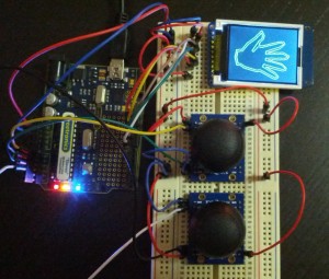
On the right here is the hardware I’m using (click for a larger image). It’s an Arduino Uno connected to an 1.8″ TFT LCD display, 160 by 128 18-bit color pixels, and two 2-axis joysticks for navigating. The zooming, rotating, and panning you saw in the videos above was controlled by the joysticks: the top one pans up/down and left/right, the bottom one zooms in and out when you move it up and down and rotates when you move it left and right. I had the Arduino already and the rest, the display and joysticks, cost me around $45.
Software setup
If you open an .svg file you’ll see that path elements are specified using a graphical operation format that looks something like this
m 157.10609,48.631198
c 0,37.817019 -51.99553,51.899082 -77.682505,13.390051
C 52.802707,101.94644 2.8939181,85.209645 2.8939181,48.57149
c 0,-36.638156 49.6730159,-54.2537427 76.5296669,-13.344121
l 25.451205,-40.4365453 77.682505,-24.41472 77.682505,13.403829
z
Each line is a graphical operation: m is moveTo, c is curveTo, l is lineTo, etc. Lower-case indicates that the coordinates are relative to the endpoint of the last operation, upper-case means that the coordinates are absolute.
The first step was to get this onto the Arduino so I wrote a python script that switched to using purely absolute coordinates and output the operations as a C data structure:
The macros, move_to, curve_to, etc., insert a tag in front of the coordinates. The result is like a bytecode format that encodes the path as a sequence of doubles. The main program runs through the path and renders it, one operation at a time, onto the display. Once it’s done it starts over again.
To implement navigation there is a transformation matrix that is updated based on the state of the joysticks and multiplied onto each of the the coordinates before they’re drawn. For details of how the matrix math works see the source code on github.
This is the same basic program that runs everything, from the very basic version to the heavily optimized version you saw at the beginning – the difference is how tuned the code is.
The display comes with a library that allows you to draw simple graphics like circles, straight lines, etc., and that’s what the drawing routines were initially based on. What it doesn’t come with is an operation for drawing curves so the main challenge was to implement curve_to.
Bezier curves
The SVG curve_to operation draws a cubic Bezier curve. I’m going to assume that you already know what a Bezier curve is so this is just a reminder. A cubic Bezier curve is defined by four points: start, end, and two control points, like you see here on the right. It goes from the start point to the end point and along the way gravitates towards first the one control point, then the second one, nice and smoothly.
If you’re given four points, let’s call them , , and so on, the Bezier defined by them is given by these parametric curves in x and y for t going between 0 and 1:
I’ll spend some more time working with this definition in a bit and rather than write two equations each time, one for x and one for y, I’m going to use the 2-element vector instead so I can write:
It means the same as the x and y version but is shorter.
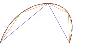
Using this definition you can draw a decent approximation of any Bezier curve just by plugging in values of t and drawing straight lines between the points you get out. The smoother you want the curve to be the more line segments you can use. On the right here is an example of using 2, 4, 8, 16, and 32 straight line segments. And on a small LCD you don’t need that many to get a decent-looking result.
First attempts
The graphics library that comes with the LCD supports drawing straight lines so it’s easy to code up the segment approach. On the right is the same video from before of what that looks like with 2 segments per curve. The way it works is that it clears the display, then draws the curve from one end to the other, and then repeats. As you can see it looks awful. It’s so slow that you can see how it constantly refreshes.
The problem is the size and depth of the display. With 160 by 128 at 18-bit colors you need 45K just to store the display buffer – and the controller only has 2K of memory. So instead of buffering the line drawing routine sends each individual pixel to the display immediately. Writing a block of data is reasonably fast (sort of, I’ll get back to that later) but writing individual pixels is painfully slow.
Luckily, for what I want to do I really don’t need full colors, monochrome is good enough, so that reduces the memory requirement dramatically. At 1-bit depth 160 by 128 pixels is still more than we can fit in memory but it’s small enough though that half does fit. So the first improvement is to buffer half the image, flush it to the display in one block, then clear the buffer, buffer the second half and then flush that.
As you can see that already looks a lot better. The biggest improvement is that there’s no need to clear the display between updates so you don’t see it refreshing at all unless you move the image. Refreshing is also a lot faster because the program takes advantage of sending whole blocks of data. But the drawing is still quite coarse, and refreshing is slow. There is also a short but visible pause between rendering the first and second half. There’s some work to do before this is good enough that you can draw something like a map of Australia from the beginning.
Faster Bezier curves
Most of the rendering time is spent computing points along the Bezier curves. For each t the program is doing a lot of work:
for (uint8_t i = 1; i <= N; i++) {
  double t = static_cast<double>(i) / N;
  Point next = (p[0] * pow(1 - t, 3))
             + (p[1] * 3 * t * pow(1 - t, 2))
             + (p[2] * 3 * pow(t, 2) * (1 - t))
             + (p[3] * pow(t, 3));
  // Draw a line from the previous point to next
}
You can be a lot smarter about calculating this. The general Bezier formula from before can be rewritten as:
where
The four Ks can be calculated just once at the beginning and then used to calculate the points along the curve in a slightly simpler way than the original formula. But there is still a lot of work going on. The thing to notice is that what we’re doing here is calculating successive values of a polynomial at fixed intervals. I happened to write a post about that problem a few months ago because that’s exactly what the difference engine was made to solve. The difference engine used divided differences to solve that problem, and we can do exactly the same.
To give a short recap of how divided differences works, if you want to calculate successive values of a n-degree polynomial, let’s take the square function, you can do it by calculating the first n+1 values,
calculate the distances between those values (the first differences) and then the distances between those (the second difference),
You can then calculate successive values of the polynomial using only addition, by adding together the differences:
You don’t need the full table either, just the last of each of the differences:
We can do the same with the Bezier, except that it’s order 3 so we need 4 values and 3 orders of differences:
Point d0 = /* The same formula as above for t=0.0 */
Point d1 = /* ... and t=(1.0/N) */
Point d2 = /* ... and t=(2.0/N) */
Point d3 = /* ... and t=(3.0/N) */// Calculate the differences
d3 = d3 - d2;
d2 = d2 - d1;
d1 = d1 - d0;
d3 = d3 - d2;
d2 = d2 - d1;
d3 = d3 - d2;
// Draw the segmentsfor (uint8_t i = 1; i <= N; i++) {
d0 = d0 + d1;
d1 = d1 + d2;
d2 = d2 + d3;
Point next = d0;
// Draw a line from the previous point to next
}
For each loop D0 will hold the next point along the curve. That’s not bad. At this point we’re only doing a constant amount of expensive work at the beginning to get the four Di and the rest is simple addition. It would be great through if we could get rid of more of the expensive work, and we can.
Let’s say we want n line segments per curve, and let’s define . Then the first four values we need for the differences are:
That makes the four differences:
This means that instead of calculating the full values and the subtracting them from each other we can plug in the four points to calculate the Ks and then use them to calculate the Ds. Coding this is straightforward too:
staticconstdouble d = 1.0 / N;
// Calculate the four ks.
Point k0 = p[0];
Point k1 = (p[1] - p[0]) * 3;
Point k2 = (p[2] - p[1] * 2 + p[0]) * 3;
Point k3 = p[3] - p[2] * 3 + p[1] * 3 - p[0];
// Calculate the four ds.
Point d0 = k0;
Point d1 = (((k3 * d) + k2) * d + k1) * d;
Point d2 = ((k3 * (3 * d)) + k2) * (2 * d * d);
Point d3 = k3 * (6 * d * d * d);
// ... the rest is exactly the same as above
This makes the initial step somewhat less expensive. But it turns out that we can get rid of the initial computation completely if we’re willing to fix the number of segments per curve at compile time.
Transformations
Even better than calculating the Ki and Di for each curve while running would be if we could calculate the Di ahead of time and store those instead of the Pi. That way we would only need to do the additions, there would be no multiplication at all involved in calculating the line segments. It should be easy – the Ds only depend on n (through d) and the Ps and all those are known at compile time.
Well actually no because it’s not the compile time known Ps that are being used here, it’s the result of multiplying them with the view matrix, which is how navigation is implemented. And that matrix is calculated based on input from the joysticks so it’s as compile time unknown as it could possibly be.
The matrix transformation itself is simple, it produces a from a by doing:
which I’ll write as
where M is a 3 by 2 matrix. That doesn’t mean that precomputing the Ds is impossible though. If you plug the definition of P’ into the definitions of the Ks and Ds it’s trivial to see that the post-transformation D0, , is simply
It takes a bit more work for the other Ds but it turns out that for all of them it holds that:
Where is the same as except that the constant factor is left out. So
is defined as
So you can precompute the Ds and still navigate the image if you just apply the transformation matrix slightly differently. And calculating the Ds is simple enough that it can be made a compile time constant if the Ps are compile time constant, which they are.
With this change the curve drawing routine becomes trivial:
// Read the precomputed ds into local variables
Point d0 = d[0];
Point d1 = d[1];
Point d2 = d[2];
Point d3 = d[3];
// Draw the segmentsfor (uint8_t i = 1; i <= N; i++) {
d0 = d0 + d1;
d1 = d1 + d2;
d2 = d2 + d3;
Point next = d0;
// Draw a line from the previous point to next
}
If you compare this with the initial implementation this looks very tight, it’s hard to imagine how you can improve upon drawing parametric curves using only addition. But there is one place.
The thing is, all these additions are done on floating-point numbers and the Arduino only has software support for floating-point, not native. So even if it’s only addition it’s still relatively expensive. The last step will be to change this to using pure integers.
Fixed point numbers
The display I’m drawing this on is quite small so the the numbers that are involved are quite small too. A 32-bit float gives much more precision than we need. Instead we’ll switch to using fixed-point numbers. It’s pretty straightforward actually. Any floating-point value in the input you multiply by a large constant, in this case I’ll use 216, and then rounded the result to a 32-bit integer. Then you do all the arithmetic on that integer, replacing floating-point addition, multiplication and division by constants, etc., with the corresponding integer operations. Finally just before rendering any coordinates on the display you divide by the constant, this time by left-shifting by 16, and the result will be very close to the same as you’d have gotten using floating point. You can get it close enough that the difference isn’t visible. And even though the Arduino doesn’t have native support for 32-bit integers either they’re still a lot faster than floats.
Multiplying by 216 means that we can represent values between -32768 and 32767, with a fixed accuracy of around 10-5. That turns out to be plenty of range for any number we need for this size display even at the max zoom level but the accuracy is slightly too low as you can see in this video:
When going from floating to fixed point directly you end up with these visible artifacts. There is a relatively simple fix for that though. The problem is caused by these two, the precomputed values of D2 and D3:
In both cases we’re calculating a value and then dividing it by a large number, the number of segments per curve squared and cubed respectively. Later on, especially when you zoom in, you’re multiplying them with a large number which magnifies the inaccuracy enough that it becomes visible. The solution is to not divide by those constants until after the matrix transformation. That makes the artifacts go away. It’s a little more work at runtime but at the point where we’re doing it we’re working with integers so if N is a power of 2 the division is actually a shift.
At this point the slowest part is shipping the data to the LCD. It turns out there were some opportunities to improve that as well so the very last step is to do that.
Faster serial
The data connection to the display is serial so every single bit goes over just a single pin using SPI. The Arduino has hardware support for SPI on a few pins so that’s what I’m using. The way you use the hardware support from C code is like this (where c is a uint8_t):
SPDR = c;
while (!(SPSR & (1 << SPIF)))
  ;
You store the byte you want to send at a particular address and then wait for the signal that the transfer is done by waiting for a particular bit to be set at a different address. We’re doing this for each byte so that’s a lot of busy waiting for that bit to flip. The first improvement is to flip them around,
while (!(SPSR & (1 << SPIF)))
  ;
SPDR = c;
Now instead of waiting before continuing we continue on immediately after starting the write, and then we wait for the previous SPI write to complete before starting the next one. If there is any work to be done between sending two pixels, and it does take a little work to decode the buffer and decide what to write out, we’re now doing that work first before waiting for the bit to flip.
Also, a great way to make sending data fast is to send less data. By default you send 18 bits per pixel but the display allows you to send only 12. In 12 bit mode you send two pixels together in 3 bytes. You switch to 12 bit mode by changing the init sequence slightly.
Patching these two changes into the underlying graphics library shaves around 25% off the time to flush to the display. It also means that you can’t just load my code and run it against the vanilla libraries but the tweaks you need are absolutely minimal.
The results
That’s it, you’ve seen every single trick I used. Here’s a longer video that shows different segment counts, from quite coarse with a decent frame rate to very smooth but somewhat slow.
When I say “decent frame rate” I don’t mean “Peter Jackson thinks this looks good”. What I mean is that the display is refreshed often enough that when you move the joysticks you get feedback quickly enough that you can actually navigate without getting lost. If it takes 500ms to refresh it becomes almost impossible, or at least really frustrating, to zoom in on a detail; if it takes 150ms it’s not a problem. And with the final version you can do that even at 32 segments per curve. It’s not super pretty but fast enough that using the navigation is not a problem.
If you were so inclined you could squeeze this even more especially if you get a parallel rather than a serial connection to the display to get the flush delay down. The reason I’m actually playing around with Bezier curves is for a different project with different components and those remaining improvements won’t help me for that. But with a parallel connection I do suspect you can get the frame rate as high as 20 FPS with this setup. I’ll leave that to someone else though.
This post is an appendix to my previous post about 0x5f3759df. It probably won’t make sense if you haven’t read that post (and if you’ve already had enough of 0x5f3759df you may consider skipping this one altogether).
One point that bugged me about the derivation in the previous post was that while it explained the underlying mathematics it wasn’t very intuitive. I was basically saying “it works because of, umm, math“. So in this post I’ll go over the most abstract part again (which was actually the core of the argument). This time I’ll explain the intuition behind what’s going on. And there’ll be some more graphs. Lots of them.
The thing is, there is a perfectly intuitive explanation for why this works. The key is looking more closely at the float-to-int bit-cast operation. Let’s take that function,
int float_to_int(float f) {
  return *(int*)&f;
}
and draw it as a graph:
This is a graph of the floating-point numbers from around 1 to 10 bit-cast to integers. These are very large integers (L is 223 so 128L is 1 073 741 824). The function has visible breaks at powers of two and is a straight line inbetween. This makes sense intuitively if you look at how you decode a floating-point value:
The mantissa increases linearly from 0 to 1; those are the straight lines. Once the mantissa reaches 1 the exponent is bumped by 1 and the mantissa starts over from 0. Now it’ll be counting twice as fast since the increased exponent gives you another factor of 2 multiplied onto the value. So after a break the straight line covers twice as many numbers on the x axis as before.
Doubling the distance covered on the x axis every time you move a fixed amount on the y axis – that sounds an awful lot like log2. And if you plot float_to_int and log2 (scaled appropriately) together it’s clear that one is an approximation of the other.
In other words we have that
This approximation is just a slightly different way to view the linear approximation we used in the previous post. You’ll notice that the log2 graph overshoots float_to_int in most places, they only touch at powers of 2. For better accuracy we’ll want to move it down a tiny bit – you’ll already be familiar with this adjustment: it’s σ. But I’ll leave σ out of the following since it’s not strictly required, it only improves accuracy.
You can infer the approximation formula from the above formula alone but I’ll do it slightly differently to make it easier to illustrate what’s going on.
The blue line in the graph above, float_to_int(v), is the i in the original code and the input to our calculation. We want to do integer arithmetic on that value such we get an output that is approximately
the integer value that, if converted back to a float, gives us roughly the inverse square root of x. First, let’s plot the input and the desired output in a graph together:
The desired output is decreasing because it’s a reciprocal so the larger the input gets the smaller the output. They intersect at v=1 because the inverse square root of 1 is 1.
The first thing we’ll do to the input is to multiply it by -1 to make it decrease too:
Where before we had a very large positive value we now have is a very large negative one. So even though they look like they intersect they’re actually very far apart and on different axes: the left one for the desired output, the right one for our work-in-progress approximation.
The new value is decreasing but it’s doing it at a faster rate than the desired output. Twice as fast in fact. To match the rates we multiply it by 1/2:
Now the two graphs are decreasing at the same rate but they’re still very far apart: the target is still a very large positive value and the current approximation is a half as large negative value. So as the last step we’ll add 1.5LB to the approximation, 0.5LB to cancel out the -1/2 we multiplied it with a moment ago and 1LB to bring it up to the level of the target:
And there it is: a bit of simple arithmetic later and we now have a value that matches the desired output:
The concrete value of the constant is
Again the approximation overshoots the target slightly the same way the log2 approximation did before. To improve accuracy you can subtract a small σ from B. That will give a slightly lower constant – for instance 0x5f3759df.
And with that I think it’s time to move onto something else. I promise that’s the last you’ll hear from me on the subject of that constant.
This post is about the magic constant 0x5f3759df and an extremely neat hack, fast inverse square root, which is where the constant comes from.
Meet the inverse square root hack:
float FastInvSqrt(float x) {
  float xhalf = 0.5f * x;
  int i = *(int*)&x;         // evil floating point bit level hacking
  i = 0x5f3759df - (i >> 1);  // what the fuck?
  x = *(float*)&i;
  x = x*(1.5f-(xhalf*x*x));
  return x;
}
What this code does is calculate, quickly, a good approximation for
It’s a fairly well-known function these days and first became so when it appeared in the source of Quake III Arena in 2005. It was originally attributed to John Carmack but turned out to have a long history before Quake going back through SGI and 3dfx to Ardent Computer in the mid 80s to the original author Greg Walsh. The concrete code above is an adapted version of the Quake code (that’s where the comments are from).
This post has a bit of fun with this hack. It describes how it works, how to generalize it to any power between -1 and 1, and sheds some new light on the math involved.
(It does contain a fair bit of math. You can think of the equations as notes – you don’t have to read them to get the gist of the post but you should if you want the full story and/or verify for yourself that what I’m saying is correct).
Why?
Why do you need to calculate the inverse of the square root – and need it so much that it’s worth implementing a crazy hack to make it fast? Because it’s part of a calculation you do all the time in 3D programming. In 3D graphics you use surface normals, 3-coordinate vectors of length 1, to express lighting and reflection. You use a lot of surface normals. And calculating them involves normalizing a lot of vectors. How do you normalize a vector? You find the length of the vector and then divide each of the coordinates with it. That is, you multiply each coordinate with
Calculating is relatively cheap. Finding the square root and dividing by it is expensive. Enter FastInvSqrt.
What does it do?
What does the function actually do to calculate its result? It has 4 main steps. First it reinterprets the bits of the floating-point input as an integer.
int i = *(int*)&x; // evil floating point bit level hack
It takes the resulting value and does integer arithmetic on it which produces an approximation of the value we’re looking for:
i = 0x5f3759df - (i >> 1); // what the fuck?
The result is not the approximation itself though, it is an integer which happens to be, if you reinterpret the bits as a floating point number, the approximation. So the code does the reverse of the conversion in step 1 to get back to floating point:
x = *(float*)&i;
And finally it runs a single iteration of Newton’s method to improve the approximation.
x = x*(1.5f-(xhalf*x*x));
This gives you an excellent approximation of the inverse square root of x. The last part, running Newton’s method, is relatively straightforward so I won’t spend more time on it. The key step is step 2: doing arithmetic on the raw floating-point number cast to an integer and getting a meaningful result back. That’s the part I’ll focus on.
What the fuck?
This section explains the math behind step 2. (The first part of the derivation below, up to the point of calculating the value of the constant, appears to have first been found by McEniry).
Before we can get to the juicy part I’ll just quickly run over how standard floating-point numbers are encoded. I’ll just go through the parts I need, for the full background wikipedia is your friend. A floating-point number has three parts: the sign, the exponent, and the mantissa. Here’s the bits of a single-precision (32-bit) one:
s e e e e e e e e m m m m m m m m m m m m m m m m m m m m m m m
The sign is the top bit, the exponent is the next 8 and the mantissa bottom 23. Since we’re going to be calculating the square root which is only defined for positive values I’m going to be assuming the sign is 0 from now on.
When viewing a floating-point number as just a bunch of bits the exponent and mantissa are just plain positive integers, nothing special about them. Let’s call them E and M (since we’ll be using them a lot). On the other hand, when we interpret the bits as a floating-point value we’ll view the mantissa as a value between 0 and 1, so all 0s means 0 and all 1s is a value very close to but slightly less than 1. And rather than use the exponent as a 8-bit unsigned integer we’ll subtract a bias, B, to make it a signed integer between -127 and 128. Let’s call the floating-point interpretation of those values e and m. In general I’ll follow McEniry and use upper-case letters for values that relate to the integer view and and lower-case for values that relate to the floating-point view.
Converting between the two views is straightforward:
For 32-bit floats L is 223 and B is 127. Given the values of e and m you calculate the floating-point number’s value like this:
and the value of the corresponding integer interpretation of the number is
Now we have almost all the bits and pieces I need to explain the hack so I’ll get started and we’ll pick up the last few pieces along the way. The value we want to calculate, given some input x, is the inverse square root or
For reasons that will soon become clear we’ll start off by taking the base 2 logarithm on both sides:
Since the values we’re working with are actually floating-point we can replace x and y with their floating-point components:
Ugh, logarithms. They’re such a hassle. Luckily we can get rid of them quite easily but first we’ll have to take a short break and talk about how they work.
On both sides of this equation we have a term that looks like this,
where v is between 0 and 1. It just so happens that for v between 0 and 1, this function is pretty close to a straight line:
Or, in equation form:
Where σ is a constant we choose. It’s not a perfect match but we can adjust σ to make it pretty close. Using this we can turn the exact equation above that involved logarithms into an approximate one that is linear, which is much easier to work with:
Now we’re getting somewhere! At this point it’s convenient to stop working with the floating-point representation and use the definitions above to substitute the integer view of the exponent and mantissa:
If we shuffle these terms around a few steps we’ll get something that looks very familiar (the details are tedious, feel free to skip):
After this last step something interesting has happened: among the clutter we now have the value of the integer representations on either side of the equation:
In other words the integer representation of y is some constant minus half the integer representation of x. Or, in C code:
i = K - (i >> 1);
for some K. Looks very familiar right?
Now what remains is to find the constant. We already know what B and L are but we don’t have σ yet. Remember, σ is the adjustment we used to get the best approximation of the logarithm, so we have some freedom in picking it. I’ll pick the one that was used to produce the original implementation, 0.0450465. Using this value you get:
Want to guess what the hex representation of that value is? 0x5f3759df. (As it should be of course, since I picked σ to get that value.) So the constant is not a bit pattern as you might think from the fact that it’s written in hex, it’s the result of a normal calculation rounded to an integer.
But as Knuth would say: so far we’ve only proven that this should work, we haven’t tested it. To give a sense for how accurate the approximation is here is a plot of it along with the accurate inverse square root:
This is for values between 1 and 100. It’s pretty spot on right? And it should be – it’s not just magic, as the derivation above shows, it’s a computation that just happens to use the somewhat exotic but completely well-defined and meaningful operation of bit-casting between float and integer.
But wait there’s more!
Looking at the derivation of this operation tells you something more than just the value of the constant though. You will notice that the derivation hardly depends on the concrete value of any of the terms – they’re just constants that get shuffled around. This means that if we change them the derivation still holds.
First off, the calculation doesn’t care what L and B are. They’re given by the floating-point representation. This means that we can do the same trick for 64- and 128-bit floating-point numbers if we want, all we have to do is recalculate the constant which it the only part that depends on them.
Secondly it doesn’t care which value we pick for σ. The σ that minimizes the difference between the logarithm and x+σ may not, and indeed does not, give the most accurate approximation. That’s a combination of floating-point rounding and because of the Newton step. Picking σ is an interesting subject in itself and is covered by McEniry and Lomont.
Finally, it doesn’t depend on -1/2. That is, the exponent here happens to be -1/2 but the derivation works just as well for any other exponent between -1 and 1. If we call the exponent p (because e is taken) and do the same derivation with that instead of -1/2 we get:
Let’s try a few exponents. First off p=0.5, the normal non-inverse square root:
or in code form,
i = 0x1fbd1df5 + (i >> 1);
Does this work too? Sure does:
This may be a well-known method to approximate the square root but a cursory google and wikipedia search didn’t suggest that it was.
It even works with “odd” powers, like the cube root
which corresponds to:
i = (int) (0x2a517d3c + (0.333f * i));
Since this is an odd factor we can’t use shift instead of multiplication. Again the approximation is very close:
At this point you may have noticed that when changing the exponent we’re actually doing something pretty simple: just adjusting the constant by a linear factor and changing the factor that is multiplied onto the integer representation of the input. These are not expensive operations so it’s feasible to do them at runtime rather than pre-compute them. If we pre-multiply just the two other factors:
we can calculate the value without knowing the exponent in advance:
i = (1 - p) * 0x3f7a3bea + (p * i);
If you shuffle the terms around a bit you can even save one of multiplications:
i = 0x3f7a3bea + p * (i - 0x3f7a3bea);
This gives you the “magic” part of fast exponentiation for any exponent between -1 and 1; the one piece we now need to get a fast exponentiation function that works for all exponents and is as accurate as the original inverse square root function is to generalize the Newton approximation step. I haven’t looked into that so that’s for another blog post (most likely for someone other than me).
The expression above contains a new “magical” constant, 0x3f7a3bea. But even if it’s in some sense “more magical” than the original constant, since that can be derived from it, it depends on an arbitrary choice of σ so it’s not universal in any way. I’ll call it Cσ and we’ll take a closer look at it in a second.
But first, one sanity check we can try with this formula is when p=0. For a p of zero the result should always be 1 since x0 is 1 independent of x. And indeed the second term falls away because it is multiplied by 0 and so we get simply:
i = 0x3f7a3bea;
Which is indeed constant – and interpreted as a floating-point value it’s 0.977477 also known as “almost 1” so the sanity check checks out. That tells us something else too: Cσ actually has a meaningful value when cast to a float. It’s 1; or very close to it.
That’s interesting. Let’s take a closer look. The integer representation of Cσ is
This is almost but not quite the shape of a floating-point number, the only problem is that we’re subtracting rather than adding the second term. That’s easy to fix though:
Now it looks exactly like the integer representation of a floating-point number. To see which we’ll first determine the exponent and mantissa and then calculate the value, cσ. This is the exponent:
and this is the mantissa:
So the floating-point value of the constant is (drumroll):
And indeed if you divide our original σ from earlier, 0.0450465, by 2 you get 0.02252325; subtract it from 1 you get 0.97747675 or our friend “almost 1” from a moment ago. That gives us a second way to view Cσ, as the integer representation of a floating-point number, and to calculate it in code:
Note that for a fixed σ these are all constants and the compiler should be able to optimize this whole computation away. The result is 0x3f7a3beb – not exactly 0x3f7a3bea from before but just one bit away (the least significant one) which is to be expected for computations that involve floating-point numbers. Getting to the original constant, the title of this post, is a matter of multiplying the result by 1.5.
With that we’ve gotten close enough to the bottom to satisfy at least me that there is nothing magical going on here. For me the main lesson from this exercise is that bit-casting between integers and floats is not just a meaningless operation, it’s an exotic but very cheap numeric operation that can be useful in computations. And I expect there’s more uses of it out there waiting to be discovered.
(Update: I’ve added an appendix about the intuition behind the part where I shuffle around the floating-point terms and the integer terms appear.)
Many (most?) virtual machines for dynamically typed languages use tagged integers. On a 32-bit system the “natural” tagsize for a value is 2 bits since objects are (or can easily be) 4-byte aligned. This gives you the ability to distinguish between four different types of values each with 30 bits of data, or three different types where two have 30 bits and one has 31 bits of data. V8 uses the latter model: 31 bit integers, 30 bit object pointers and 30 bit “failure” pointers used for internal bookkeeping. On 64-bit systems the natural tagsize is 3 which allows for more types of tagged values, and inspired by this I’ve been playing around with tagging another kind of value: double precision floating-point numbers.
Whenever you want to tag a value you need to find space in the value for the tag. With objects it’s easy: they’re already aligned so the lowest few bits are automatically free:
With integers no bits are free automatically so you only tag if the highest bits are the same, by shifting the lowest bits up and adding the tag in the lowest bits, for instance:
The reason both the highest bits 0000 and 1111 work is that when you shift up by 3 there will be one bit of the original 4 left, and when shifting down again sign extension spreads that bit back out over all the top 4 bits.
With doubles it becomes harder to find free bits. A double is represented as one sign bit s, an 11-bit exponent e and a 52 bit fraction, f:
seeeeeeeeeeeffffffffff..fffffffff (untagged)
The value of the number is (-1)s2e1.f.
To get a feel for how this representation works I tried decomposing some different values into into their parts, here using single precision but the same pattern applies to double precision:
value
sign
exponent
fraction
1.0
0
0
1
-1.0
1
0
1
2.0
0
1
1
0.5
0
-1
1
3.0
0
1
1.5
100.0
0
6
1.5625
10000.0
0
13
1.2207031
-10000.0
1
13
1.2207031
0.0001
0
-14
1.6384
0
0
-127
0.0 (denormalized)
NaN
0
128
1.5
Infinity
0
128
1.0
Looking at this table it’s clear that in an interval around ±1.0, starting close to 0.0 on the one side and stretching far out into the large numbers, the exponent stays fairly small. There are 11 bits available to the exponent, that’s a range from -1022 to 1023 since one exponent is used for special values, but for all values between 0.0001 and 10000 for instance its actual value only runs from -14 to 13.
Even though the high bits of the exponent are unused for many numbers you can’t just grab them for the tag. The 11 exponent bits don’t contain the exponent directly but its value plus a bias of 1023, apparently to make comparison of doubles easier. But after subtracting the bias from the exponent it is indeed just a matter of stealing its top three bits of the value (leaving the sign bit in place):
Using this approach all doubles whose exponent is between -127 and 128 can be tagged. Since single precision numbers use 8 bits for the exponent all numbers between the numerically greatest and numerically smallest single precision numbers, positive and negative, can be represented as tagged doubles. One potential concern is that this encoding does not allow ±0.0, NaNs or ±∞ but I’m not too worried about that; it’s easy to handle 0.0 specially and it’s unclear how problematic the other values are.
What’s the performance of this? The short answer is: I don’t know, haven’t tried it. The long answer is: I can guess and I’m fairly certain that it’s worth it.
One reason it might not be worth it is if most doubles are not covered by this. To test this I instrumented v8 to test each time a heap number was allocated whether the value would fit as a tagged double. Furthermore I disabled some optimizations that avoid number allocation to make sure the allocation routines saw as many numbers as possible. The results after running the v8 benchmarks were encouraging:
The number in c:SmallDoubleHits is the ones that fit in a tagged double: 92%. Furthermore, of the numbers that could not be represented all but 2% were zero or infinity. The v8 benchmark suite contains two floating-point heavy benchmarks: a cryptography benchmark and a raytracer. Interestingly, the cryptography benchmarks is responsible for almost all the ∞s and the raytracer is responsible for almost all the 0.0s. If a special case was added for 0.0 then 99.3% of all the doubles used in the raytracer would not require heap allocation.
Note: peopleoftenask if we plan to add 64-bit support to v8. Don’t read this as an indication one way or the other. I’m just testing this using v8 because that’s the code base and benchmarks I know best.
Note that this is just a single data point, there’s no basis to conclude that the same holds across most applications. Note also that since v8 uses tagged integers there is some overlap between this an existing optimizations. But since all 32-bit integers can be represented as tagged doubles any nonzero numbers that are not counted because they were recognized as small integers would have counted as tagged doubles.
Another reason it might not be worth it could be that tagging and untagging is expensive; I doubt that it is considering how relatively few operations it takes:
I haven’t benchmarked this so I can only guess about the performance. I have no doubt that testing and tagging a double is faster overall than allocating a heap object but I suspect reading from memory could turn out to be cheaper than untagging. The overall performance also depends on how doubles are used: if most are only used briefly and then discarded then the possible cheaper reads don’t make up for the more expensive allocation. But I’m just guessing here.
In any case I think this is a promising strawman and it would be interesting to see how it performed in a real application. I also suspect there are more efficient ways of tagging/untagging the same class of doubles. The problem is actually a fairly simple one: reduce the highest bits from 01000, 11000, 01111 or 11111 to only two bits and be able to go back again to the same five bits.
Further reading: alternative approaches are here, which is essentially the same as this but has more special cases, and this which goes the other way and stores other values in the payload of NaN values.
I’ve recently gone from being indifferent to varargs in C++ to thinking that they should be avoided at all cost. It’s a collection of values (but not references or objects passed by value) that you don’t know the length or type of, that you can’t pass on directly to other variadic functions, and that can only be streamed over not accessed randomly. Bleh! In the case of printf-like function, which I expect is the most popular use of varargs, you add the information that is missing from the arguments themselves to the format string. This gives ample opportunity for mistakes, which some compilers will warn you of but which other’s won’t. For me, the conclusion has been that varargs are harmful and should not be used under any circumstances.
Of course, not having printf-like functions in C++ is a drag if you want to build strings so I’ve been trying to come up with something to replace it that isn’t too painful. What the remainder of this post is about is that you can actually have your cake and eat it too: you can have something that looks just like printf that doesn’t use varargs but takes a variable (but bounded) number of arguments where the arguments each carry their own type information and can be accessed randomly. Where you would write this using classic printf:
int position = ...; constchar *value = ...; printf("Found %s at %i", value, position);
this is how it looks with dprintf (dynamically typed printf):
dprintf("Found % at %", args(value, position))
You’ll notice that dprintf is different from printf in that:
There is no type information in the format string; arguments carry their own type info. Alternatively you could allow type info in the format string and use the info carried by the arguments for checking.
The arguments are wrapped in a call to args. This is the price you have to pay syntactically.
To explain how this works I’ll take it one step at a time and start with how to automatically collect type information about arguments.
Type Tagging
When calling dprintf each argument is coupled with information about its type. This is done using implicit conversion and static overloading. If you pass an argument to a function in C++ and the types don’t match then C++ will look at the expected argument types and, if possible, implicitly convert the argument to the expected type. This implicit conversion can be used to collect type information:
call_me(4); // Prints the value of INT call_me("foo"); // Prints the value of C_STR
When calling call_me the arguments don’t match so C++ implicitly finds the int and const char* constructors of TaggedValue and calls them. Each constructor in TaggedValue does a minimal amount of processing to store the value and type info about the value. The important part here is that you don’t see this when you invoke call_me so as a user you don’t have to worry about how this works, all you know is that type info is somehow being collected.
This has the limitation that it only works for a fixed set of types, the types for which there is a constructor in TaggedValue — but on the other hand this is no different from the fixed set of formatting directives understood by printf. On the plus side it allows you to pass any value by reference and by value as long as TaggedValue knows about it in advance. The issue of automatic type tagging is actually an interesting one; in this case we only allow a fixed set of “primitive” types but there is no reason why tagging can’t work for array types or other even more complex types[1].
The next step is to allow a variable number of these tagged values. Enter the args function.
Variable argument count
This is the nastiest part of it all since we have to define an args function for every number of arguments we want to allow. This function will pack the arguments up in an object and return it to the dprintf call:
// Abstract superclass of the actual argument collection class TaggedValueCollection { public: TaggedValueCollection(int size) : size_(size) { } int size() { return size_; } virtualconst TaggedValue &get(int i) = 0; private: int size_; }
The TaggedValueCollectionImpl holds the arguments and provides access to them. The TaggedValueCollection superclass are there to allow methods to access the arguments without knowing how many there are. The number of arguments are part of the type of TaggedValueCollectionImpl so we can’t use that directly. The args function is the one that handles 3 arguments but they all look like this. It creates a new collection and stores its arguments in it. While it is bad to have to define a function for each number of arguments it is much better than varargs. Also, you only have to write these functions once, and then every function with printf-like behavior can use them.
Finally, the dprintf function looks like this:
void dprintf(string format, const TaggedValueCollection &elms) {
  // Do the formatting
}
One advantage about having random access to the arguments is that the format string can access them randomly, they don’t have to be accessed in sequence. I’ve used the syntax $i to access the i‘th argument:
dprintf("Reverse order (2: $2, 1: $1, 0: $0)", args("a", "b", "c"))
// -> prints "Reverse order (2: c, 1: b, 0: a)"
Coupled with the fact that format strings don’t have to contain type info this gives a lot more flexibility in dealing with format strings. Honestly I’ve never had any use for this but I could imagine that it could be useful for instance in internationalization where different languages have different word order.
To sum up, the advantages of this scheme are:
Type information is automatically inferred from and stored with the arguments.
You can pass any type of value by reference or by value.
The argument collections (the const TaggedValueCollection &s) can be passed around straightforwardly. You only have to define one function, there is no need for functions like vprintf.
Format strings can access arguments in random order.
I’ve switched to using this in my hobby project and it works like a charm. You can see a full implementation of this here: string.h and string.cc (see string_buffer::printf and note that the classes have different names than I’ve used here). To see how it is being used see conditions.cc for instance.
A final note: if you find this kind of thing interesting (and since you’ve come this far I expect you do) you’ll probably enjoy enjoy Danvy’s Functional Unparsing.
1: To represent more complex types you just have to be a bit more creative with how you encode the type tag. A simple scheme is to to let the lowest nibble specify the outermost type (INT, C_STR, ARRAY, …) and then, if the outermost type is ARRAY let the 28 higher bits hold the type tag of the element type. For more complex types, like pair the 28 remaining bits can be divided into two 14-bit fields that hold the type tags for T1 and T2 respectively. For instance, pair<const char*, int**> would be represented as
bits
28-31
24-27
20-23
16-19
12-15
8-11
4-7
0-3
data
c_str
int
array
array
pair
While this scheme is easy to encode and decode it can definitely be improved upon. For instance, there are many type tag values that are “wasted” because they don’t correspond to a legal type. Also, it allows you to represent some types that you probably don’t need very often while some types you are more likely to use cannot be represented. For instance, you can represent int****** but not pair<int, pair<int*, const char*>>. And of course, if you don’t have exactly 16 different cases you’re guaranteed to waste space in each nibble. But finding a better encoding is, as they say, the subject of future research.
Here’s an interesting tidbit for the code style fanatics out there. I recently found the source code of the original System 7 version of the bourne shell, sh, the father of bash. Wow. The code style is so awful that it’s almost a work of art. How bad is it? Well, I think a few lines from mac.h gives a pretty good impression:
#define IF if( #define THEN ){ #define ELSE } else { #define ELIF } elseif ( #define FI ;}
Here’s a bit of the resulting code (with pseudo-keywords highlighted):
FOR m=2*j-1; m/=2; DO k=n-m; FOR j=0; jDOFOR i=j; i>=0; i-=m DOREGSTRING *fromi; fromi = &from[i]; IF cf(fromi[m],fromi[0])>0 THEN break; ELSESTRING s; s=fromi[m]; fromi[m]=fromi[0]; fromi[0]=s; FI OD OD OD
As they would say over at the daily WTF: My eyes! The goggles do nothing! It’s C code alright, but not C code as we know it. It’s known as Bournegol, since it’s inspired by Algol. By the way, IOCCC, the International Obfuscated C Code Contest, was started partly out of disgust with this code.
So, It’s been a month and a half since I last posted anything. It’s not that I’ve given up writing here it’s just that half of what I’m doing these days I’m not allowed to tell anyone and the other half I’m too busy doing to write about. However, I fell across a useful compiler implementation technique that I thought I’d take the effort to write about. It has to do with abstract syntax trees pretending to be bytecode (and vice versa).
I am, as usual, playing around with a toy language — the second one since neptune died. This time I thought I’d shake things up a little and implement both the compiler and runtime it in C++ rather than Java. My first attempt at a compiler was straightforward: the parser read the source and turned it into a syntax tree, the syntax tree was used to generate bytecode, the bytecode was executed by the runtime.
It turns out, however, that the obvious approach is pretty far from optimal. The compiler is really stupid and doesn’t actually use the syntax tree except to do a simple recursive traversal when generating the bytecode. On the other hand, the syntax tree would be really handy if I wanted to JIT compile the code at runtime, but at that point it is long gone and there is only the bytecode left.
I tried out different approaches to solving this problem and ended up with something that is a combination of bytecode and syntax trees. In particular, it has the advantages of both bytecode and syntax trees at the cost of a small overhead. Here’s an example. The code:
def main() {
  if (1 < 2) return a + b;
  else Console.println("Huh?");
}
It it essentially a bytecode format with some extra information that allows you to reconstruct the syntax tree. A bytecode interpreter would execute it by starting at instruction 0 and ignoring the extra structural information:
On the other hand, if you want to reconstruct the syntax tree you can read the code backwards, starting from the last instruction. In this case the last instruction says that the preceding code was generated from a statement block with two statements, the ones ending at 39 and 47. If you then jump to position 39 you can see that the code ending there was generated from an if statement with the condition ending at 4, the then-part ending at 24 and the else-part ending at 32. Just like an interpreter would ignore the extra structural information, a traversal will ignore the instructions that carry no structural information such as goto and pop:
Here I’ve tried to illustrate the way the instructions point backwards using puny ASCII art. Anyway, you get the picture.
When you want to traverse the syntax tree embedded is a piece of code you don’t actually have to materialize it. Using magical and mysterious features of C++ you can create a visitor that gives the appearance of visiting a proper syntax tree when it’s really just traversing the internal pointers in one of these chunks of syntax-tree-/byte-code.
Pretty neat, I think. Having a closed syntax tree format (by which I mean one that doesn’t use direct memory pointers) means that you can let it flow from the compiler into the runtime, so you can dynamically inspect the syntax tree for a piece of code. It’s also easy to save in a binary file or send over the network.
More importantly it allows syntax trees to flow from running programs back into the compiler at runtime. One of the things I’m experimenting with this time is metaprogramming and representing code as data. In particular, I’m going for something in the style of MetaML but with dynamic rather than static typing. For that, this format will be very handy.
I’m considering reimplementing part of my Java parser library, hadrian. At the lowest level, hadrian is essentially a virtual machine with an unusual instruction set and it parses input by interpreting parser bytecodes. One thing I’ve been thinking about is replacing this simple interpreter with something a bit more clever, for instance dynamically generated java bytecode. Today I decided to play around with this approach to see how complicated that would be and how much performance there is to gain by replacing a simple bytecode interpreter loop with a dynamically generated interpreter.
Instead of actually replacing the hadrian interpreter I thought I’d do something simpler. I made a class, Handler, with one method for each letter in the alphabet, each one doing something trivial:
class Handler { private int value; publicvoid doA() { value += 1; } publicvoid doB() { value -= 1; } publicvoid doC() { value += 2; } ... }
The exercise was: given a piece of “code” in the form of a text string containing capital letters, how do you most efficiently “interpret” this string and call the corresponding methods on a handler object. Or, to be more specific, how do you efficiently interpret this string not just once but many many times. If this can be done efficiently then it should be possible to apply the same technique to a real bytecode interpreter that does something useful, like the one in hadrian.
The straightforward solution is to use an interpreter loop that dispatches on each letter and calls the corresponding method on the handler:
void interpret(char[] code, Handler h) {
  for (int i = 0; i < code.length; i++) {
    switch (code[i]) {
      case 'A': h.doA(); break;
      case 'B': h.doB(); break;
      case 'C': h.doC(); break;
      ...
    }
  }
}
That’s very similar to what hadrian currently has and it’s actually relatively efficient. It should be possible to do better though.
Java allows you to generate and load classes at runtime, but to be able to use this I had to write a small classfile assembler. There are frameworks out there for generating classfiles but I wanted something absolutely minimal, something that did just what I needed and nothing else. I found the classfile specification and wrote some code that generated a legal but empty class file that could be loaded dynamically. Surprisingly, it only took around 200 lines of code to get that working. Adding a simple bytecode assembler to that, so that I could generate methods, got it up to around 600 lines of code. That was still a lot less code than I had expected.
The simplest approach I could think of was to generate code that consisted of a sequence of calls to static methods, one static method for each “opcode” or in this case letter in the alphabet. Given a set of methods:
This means that instead of dispatching while running the code, you dispatch while generating code:
for (int i = 0; i < code.length; i++) {
  gen.aload(0); // Load first argument
  String name = "handle" + code[i];
  Method method = getDeclaredMethod(name, Handler.class);
  gen.invokestatic(method); // Call handler
}
I tried this and compared it with the simple interpreter it is, perhaps not surprisingly, quite a bit faster than the simple interpreter. On short strings, around 10-30 letters, it is around twice as fast as the interpreter. On longer strings, say 200-300 letters, it is 4-5 times faster. Nice.
I though it might be interesting to see where the theoretical limit was for this so the next thing I tried was to remove all overhead. Instead of generating calls, I generated code that performed the operations directly without going through any methods:
This was a bit more complicated to implement but I got it up and running and surprisingly, it was exactly as fast as the previous experiment. Even though there were two calls for each opcode in the previous example, one to handleX and one to h.doX, the VM apparently inlines everything. This means that you can generate efficient straight-line code simply by having a static method for each bytecode, generating a sequence of calls to those methods and then leaving the rest to the VM. And generating classfiles containing straightforward code like that can be done efficiently in very few lines of java code. If I do end up reimplementing part of hadrian, I’m sure I’ll use this technique.
I also played around with various ways of adding arguments to the generated code, like:
void run(Handler h, int x, int y) {
  handleK(h, x, y);
  handleB(h, x, y);
  handleQ(h, x, y);
  ...
}
It turns out that as soon as you add arguments, each opcode becomes twice as expensive to execute. I tried the same with the interpreter and there was no notable change in performance. But it should be possible to pack any state you need to carry around into the one argument that can be passed around without losing performance.
All in all I would say that this technique has a lot of potential, and I suspect it might have other applications than bytecode interpreters. I’m currently considering cleaning up the code and publishing it on google project hosting.
Update
This code now lives at googlecode, along with an example. The interface is pretty straightforward, especially for expressing bytecode. Here’s how this code:
public int call(int x) {
  while (x < 15)
    x = Main.twice(x);
  return x;
}
The only annoyance is that some opcode names like return and goto are reserved so I have to use names like rethurn and ghoto, following the “silent h” renaming convention.
Over on his blog, Gilad is having fun with parser combinators in smalltalk. Through the magic of smalltalk you can define a domain-specific language and then write parsers directly in the source code. For instance, this grammar
I won’t explain what it means, you should go read Gilad’s post for that.
Back before I wrote my master’s thesis (about dynamically extensible parsers) I actually wrote a simple prototype in squeak and, as you can see, smalltalk is fantastically well suited for this kind of stuff. So I thought, what the heck, maybe I’ll write a little parser combinator framework in squeak myself. So I did. Here’s a few thoughts about squeak and parser combinators.
Left recursion
Gilad mentions that you can’t express left recursive grammars directly using parser combinators. For instance, you can’t write
 :=  *
        |  /
        |  +
        |  -
        |
because must not occur on the far left side of a production in its own definition. But there are actually relatively few uses for left recursive productions and rather than restructuring the grammar to avoid left recursion you can add a few combinators to the framework that handle 95% of all uses for this. One place where you often see left recursive grammars is lists of elements separated by a token:
-> "," |
This pattern is used so often that it makes sense to introduce plus and star combinators that take an argument, a separator that must occur between terms:
exprList
  ^ (self expr) star: (self delim: ',')
The other and most complicated use of left recursion is operator definitions but that can also be expressed pretty directly in smalltalk with a dedicated combinator:
This construct takes an “atomic” term, that’s the kind of term that can occur between the operators, and then defines the set of possible operators. The result is a parser that parses the left recursive expression grammar from before. You can also expand this pattern to allow precedence and associativity specifications:
It does take a bit of doesNotUnderstand magic to implement this but the result is a mechanism that kicks ass compared to having to restructure the grammar or define a nonterminal for each level in the precedence hierarchy. Also, it can be implemented very efficiently.
Squeak
It’s been a few months since I last used squeak and it seems like a lot has happened, especially on the UI side. I think squeak is an impressive system but in some areas it’s really an intensely poorly designed platform. That probably goes all the way back to the beginning of smalltalk.
The big overriding problem is, of course, that squeak insists on owning my source code. I’m used to keeping my source code in text files. I’m happy to let tools manage them for me like eclipse does but I want the raw text files somewhere so that I can create backups, put them under version control, etc. With squeak you don’t own your source code. When you enter a method it disappears into a giant soup of code. This is a problem for me in and of itself but it’s especially troubling if you’re unfortunate enough to crash the platform. That’s what happened to me: I happened to write a non-terminating method which froze the platform so that I had to put it down. That cost me all my code. No, sorry, that cost me its code. The worst part is that I know that smalltalkers think this ridiculous model is superior to allowing people to manage their own source code. Well, you’re wrong. It’s not that I like large source files, but I want to have some object somewhere outside the platform that contains my code and that I have control over. And yes I know about file out, that’s not what I’m talking about.
Another extremely frustrating issue is that squeak insists that you write correct code. In particular you’re not allowed to save a method that contains errors. I think it’s fine to notify me when I make an error. Sometimes during the process of writing code you may, say, refer to a class or variable before it has been defined or you may briefly have two variables with the same name. I don’t mind if the system tells me about that but squeak will insist that you change your code before you can save it. The code may contain errors not because it’s incorrect but because it’s incomplete. Squeak doesn’t care. I used another system like that once, the mjølner beta system, which was intensely disliked by many of us for that very reason.
This is just one instance of the platform treating you like you’re an idiot. Another instance is the messages. If you select the option to rename a method the option to cancel isn’t labelled cancel, no, it’s labeled Forget it — do nothing — sorry I asked. Give. Me. A. Break.
All in all, using squeak again was a mixed experience. As the parser combinator code shows smalltalk the language is immensely powerful and that part of it was really fun. But clearly the reason smalltalk hasn’t conquered the world is not just that back in the nineties, Sun convinced clueless pointy-haired bosses that they should use an inferior language like Java instead of smalltalk. It’s been a long time since I’ve used a programming language as frustrating as Squeak smalltalk. On the positive side, though, most of the problems are relatively superficial (except for the file thing) and if they ever decide to fix them I’ll be happy to return.

") ,
, ") , and so on, the Bezier defined by them is given by these parametric curves in x and y for t going between 0 and 1:
, and so on, the Bezier defined by them is given by these parametric curves in x and y for t going between 0 and 1: = x_0(1-t)^3 + 3x_1t(1-t)^2 + 3x_2t^2(1-t) + x_3t^3")
 = y_0(1-t)^3 + 3y_1t(1-t)^2 + 3y_2t^2(1-t) + y_3t^3")
") instead so I can write:
instead so I can write: = P_0(1-t)^3 + 3P_1t(1-t)^2 + 3P_2t^2(1-t) + P_3t^3")
 Using this definition you can draw a decent approximation of any Bezier curve just by plugging in values of t and drawing straight lines between the points you get out. The smoother you want the curve to be the more line segments you can use. On the right here is an example of using 2, 4, 8, 16, and 32 straight line segments. And on a small LCD you don’t need that many to get a decent-looking result.
 = K_0 + K_1t + K_2t^2 + K_3t^3")

")
")


 . Then the first four values we need for the differences are:
 = K_0")
=K_0+K_1d+K_2d^2+K_3d^3")
=K_0+2K_1d+4K_2d^2+8K_3d^3")
=K_0+3K_1d+9K_2d^2+27K_3d^3")


") from a
from a ") by doing:
by doing:


 is the same as
  except that the constant factor is left out. So


")
2^e")

 \approx (\log_2(v)+B)L")
")
")
")
")
")
 \approx \frac 32LB - \frac 12 \mathtt{float\_to\_int}(v)")


 is relatively cheap. Finding the square root and dividing by it is expensive. Enter

2^e")


 + e_y = {-\frac 12}(\log_2 (1+m_x) + e_x)")
")
 vs. x + sigma")
 \approx v + \sigma")
")
")
 - \sigma + B")
 - \frac{3}{2}(\sigma - B)")
 - {\frac 12}(M_x + LE_x)")
 - {\frac 12}\mathbf{I_x}")
 = {\frac 32}2^{23}(127 - 0.0450465) = 1597463007")

L(B - \sigma) + p\mathbf{I_x}")

 = {\frac 12}2^{23}(127 - 0.0450465) = \mathtt{0x1fbd1df5}")


 = {\frac 23}2^{23}(127 - 0.0450465) = \mathtt{0x2a517d3c}")

 = 2^{23}(127 - 0.0450465) = \mathtt{0x3f7a3bea}")
 = LB - L\sigma")
 + L(1 - \sigma)")
 = (B - 1 - B) = -1")
}{L} = 1 - \sigma")
2^{e_{c_\sigma}} = \frac{1 + 1 - \sigma}2 = 1 - \frac{\sigma}2")