Monthly Archives: September 2014

I’ve been reading Learn You a Haskell and got stuck on a tiny point at the beginning, in the section about ranges: you can’t have a range with more than one step value. This post is about what it might mean to allow multiple steps and how Charles Babbage might have had an opinion on this particular aspect of haskell’s design.

Here’s the whole paragraph from Learn You a Haskell,

To make a list containing all the natural numbers from 1 to 20, you just write [1..20]. [… snip …] Ranges are cool because you can also specify a step. What if we want all even numbers between 1 and 20? Or every third number between 1 and 20?

ghci> [2,4..20]
[2,4,6,8,10,12,14,16,18,20]
ghci> [3,6..20]
[3,6,9,12,15,18]

It’s simply a matter of separating the first two elements with a comma and then specifying what the upper limit is. While pretty smart, ranges with steps aren’t as smart as some people expect them to be. You can’t do [1,2,4,8,16..100] and expect to get all the powers of 2. Firstly because you can only specify one step. And secondly because some sequences that aren’t arithmetic are ambiguous if given only by a few of their first terms.

The bold highlight is mine. This makes sense – how can the language guess that what you have in mind when you write [1, 2, 4, 8, 16..] is the powers of 2?

On the other hand though, just as a fun exercise, if you were to allow multiple step values how would you define them? Even though this is a highly specialized and modern language design question I know Charles Babbage would have understood it and I suspect he would have had an opinion.

A while ago I wrote a post about Babbage’s difference engine. The difference engine is basically an adder that calculates successive values of a polynomial by doing simple addition, using a technique called divided differences. This is described in full detail in that post but here’s a summary. Take a sequence of values of values of a polynomial, for instance the first four squares,

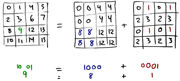
You can then calculate the next values using just addition by calculating the differences between the initial values. To get the differences for a sequence you subtract each pair of values,

Do it once and you get the first differences. Do the same thing to the first differences and you get the second differences,

Do the same thing to the second differences and you get the third differences,

In this case there’s just one and it’s 0 so we can ignore it. Once you have all the differences you can calculate the next value of the polynomial by adding them together from right to left,

There it is, 16, the next value in the sequence. At this point we can just keep going,

This technique works for any polynomial. The difference engine was given its name because it is a mechanical implementation of it.

Already you may suspect how this can be relevant to ranges in haskell. You can generalize ranges to n step values by using divided differences on the step values to generate the rest of the sequence. With two step values the result of this is a linear sequence, as you would expect (polyEnumFrom is my name for the generalized range function),

ghci> polyEnumFrom [0, 1]
[0, 1, 2, 3, 4, 5, 6, ...]
ghci> polyEnumFrom [4, 6]
[4, 6, 8, 10, 12, 14, 16, ...]
ghci> polyEnumFrom [10, 9]
[10, 9, 8, 7, 6, 5, 6, ...]


Give it three elements, for instance the squares from before, and the result is a second-order polynomial,

ghci> polyEnumFrom [0, 1, 4]
[0, 1, 4, 9, 16, 25, 36, ...]

Similarly with the cubes,

ghci> polyEnumFrom [0, 1, 8, 27]
[0, 1, 8, 27, 64, 125, 216, ...]

There is nothing magical going on here to recognize the squares or cubes here, it’s a completely mechanical process that uses subtraction to get the differences and addition to then continue the sequence past the step values. It won’t give you the squares though, only polynomials. If you try you get

ghci> polyEnumFrom [1, 2, 4, 8, 16]
[1, 2, 4, 8, 16, 31, 57, ...]

For any list of 3 step values there is exactly one polynomial of order 2 or less that yields those values; an order-2 polynomial has 3 free variables so there’s no room for more than one solution. The result of a 3-step range is the sequence of values produced by that order-2 polynomial. In general, the result of a multi-step range with n steps is the sequence of values generated by the unique polynomial of order at most n-1 whose first n values are the steps. Conveniently, if the steps are integers the polynomial is guaranteed to only produce integers.

Babbage built the difference engine because it was really important then be able to produce tables of function values by calculating successive values of polynomials. I think he would have appreciated the power of a language where you can condense the work of generating an approximate table of sine values into a single line,

take 10 (polyEnumFrom [0, 0.0002909, 0.0005818, 0.0008727])

which yields,

0.0000000
0.0002909
0.0005818
0.0008727
0.0011636
0.0014545
0.0017454
...

(The four values given to polyEnumFrom are the first four sine values from the table.) Of course, Babbage did lose interest in the difference engine himself and preferred to work on the more general analytical engine. If he did see haskell he would probably quickly lose interest in ranges and move on to more general advanced features. But I digress.

Is a shorthand for sequences of polynomial values actually a useful feature in a language? I doubt it. But I like the idea that a corner of a modern language  intersects with Babbage and the difference engine. Maybe it would make sense as a little easter-egg tribute to Babbage, a difference engine hiding behind a familiar language construct. I quite like the idea of that.

If you want to play around with it I’ve put an implementation in a gist. For something that might seem fairly complex the implementation is simple – polyEnumFrom and its helpers is just 13 lines. Haskell is an elegant language.

This is the third post in a series about z-quads, a spatial coordinate system. The first one was about the basic construction, the second about how to determine which quads contain each other. This one is about conversions: how to convert positions to quads and back.

First, a quick reminder. A quad is a square(-ish) area on the surface of the earth. Most of the time we’ll use the unit square instead of the earth because it makes things simpler and you can go back and forth between lat/longs and unit coordinates just by scaling the value up and down. (There’s a section at the end about that.)

So, when I’m talking about encoding a point as a quad, what I mean more specifically is: given a point on the unit square (x, y) and a zoom level z, find the quad at zoom level z that contains the point. As it turns out, the zoom level doesn’t really matter so we’ll always find the most precise quad for a given point. If you need a different zoom level you can just have a step at the end that gets the precise quad’s ancestor at whatever level you want.

Precision

So far we’ve focused on quads as an abstract mathematical concept and there’s been no reason to limit how far down you can zoom. In practice though you’ll want to store quads in integers of finite size, typically 32-bit or 64-bit. That limits the precision.

It turns out that you can fit 15 zoom levels into 32 bits and 31 into 64. At zoom level 15 the size of a quad is around 1.5 km². At zoom level 31 it’s around 3 cm². So yeah, you typically don’t need more than 31 levels. A third case is if you want to store your quad as a double – JavaScript, I’m looking at you here. A double can hold all integers up to 53 bits, after which some can’t be represented. That corresponds to 26 zoom levels which is also plenty precise for most uses.

Encoding points

Okay, now we’re ready to look at encoding. What we’ll do is take a unit point (x, y) and find the level 31 quad that contains it. Since we’ve fixed the zoom level we’ll immediately switch to talking about the scalar rather than the quad. That makes everything simpler because within one level we’re dealing with a normal z-order curve and conversion to and from those are well understood.

The diagram on the right illustrates something we’ve seen before: that scalars are numbered such that the children at each level are contiguous. In this example, the first two green bits say which of the four 2×2 divisions we’re in. The next two say which 1×1 subdivision of that we’re in. It’s useful to think of this the same way as the order of significance within a normal integer: the further to the left a pair of bits is in a scalar the more significant it is in determining where the scalar is.

Now things will have to get really bit-fiddly for a moment. Let’s look at just a single 2×2 division. Each subdivision can be identified with an (x, y) coordinate where each ordinate is either 0 or 1, or alternatively with a scalar from 0 to 3. The way the scalars are numbered it happens that the least significant scalar bit gives you the x-coordinate and the most significant one gives you y:

(This is by design by the way, it’s why the z-shape for scalars is convenient). This means that given point x and y, each 0 or 1, you get the scalar they correspond to by doing

x + 2 y

What’s neat about that is that because of the way pairs of bits in the scalar increase in significance from right to left matches the significance of bits in an integer, you can do this for each bit of x and y at the same time, in parallel. To illustrate how this works I’ll take an example.

Let’s start with the point (2/5, 2/3) and find the level 5 scalar that contains it. First we’ll multiply both values by 3² (=2⁵) and round the result to an integer,

x = (2/5) × 32 ≈ 12 = 01100b
y = (2/3) × 32 ≈ 21 = 10101b

Now we’ll perform x + 2 y for each bit in parallel like so,

Looks bizarre right, but it does work. We spread out the bits from each input coordinate so they can be matched up pairwise and then add them together. The result is the scalar we’re looking for because the order of significance of the bit-pairs in the scalar match the significance of the individual bits in each of the inputs.

Now, how can you tell that the result, scalar 626 on zoom level 5, is the right answer? This diagram suggests that it’s about right:

The bit-pairs in the scalar are [2, 1, 3, 0, 2]  so we first divide and take subdivision 2, then divide that and take 1, then divide that, and so on. Ultimately we end up at the green dot. In this case the last step would be to add the appropriate bias, b₅, to get a proper quad and then we’re all done.

Because this conversion handles all the levels in parallel there’s little benefit to converting to a higher zoom level than the most precise, typically 31. If you want level 5 do the conversion to level 31 and then get the 26th ancestor of the result.

Most of the work in performing a conversion is spreading out the scaled 31-bit integer coordinates. One way to spread the bits is using parallel prefix which takes log₂ n steps for an n-bit word,

  00000000abcdefgh
→ 0000abcd0000efgh
→ 00ab00cd00ef00gh
→ 0a0b0c0d0e0f0g0h

That’s just one way to do it, there are others.

Decoding quads

The operation above gets you into quad-land and obviously you’ll want to be able to get out again. This turns out to just be a matter of running the encoding algorithm backwards. The main difference is that here we’ll stay on whatever zoom level the quad’s on instead of always going to level 31.

Given a quad q this is how you’d decode it:

1. Subtract the bias to get the quad’s scalar.
2. Mask out all the even-index bits to get the spread x value and the odd-index bits to get the spread y value. Shift the y value right by 1.
3. Pack the spread-x and –y values back together to get a z_q-bit integer value for each. Packing can be similarly to spreading but in reverse.
4. Floating-point divide the integer values by 2^z_q. You now have your (x, y) coordinates between 0 and 1.

A quad is an area but the result here is a point, the top left corner of the quad. This is often what you’re interested in, for instance if you’re calculating is the full area of the quad. There you can just add the width and height of the quad (which are both 2^–z_q) to get the other corners. Alternatively you might be interested in the center of the quad instead. To get you can modify the last step of the algorithm to do,

Apply (2 v + 1) / 2^z_q+1 as a floating-point operation to each of the integer coordinates.

This is just a circuitous way to add 0.5 to v before dividing by 2^z_q but this way we can keep the value integer until the final division. If you want to minimize the loss of precision when round-tripping a point through a quad you should use the center since it’s the point with the smallest maximum distance to the points that belong to that quad.

So, now we can convert floating-point coordinates to quads and back again with ease. Well, relative ease. In the last part I’ll talk briefly about something I’ve been hand-waving until now: converting from lat/long to the unit square and back.

Latitude and longitude

When you encounter a lat/long it is typically expressed using the WGS 84 standard. The latitude, a value between -90 and 90, gives you the north-south position. The longitude, a value between -180 and 180, gives you east-west.

A typical world map will look something like the one on the right here with America to the left and Asia to the right. The top left corner, northwest of North America, is lat 90 and long -180. The bottom right, south of New Zealand, has lat -90 and long 180. You could convert those ranges to an (x, y) on the unit square in any number of ways but the way I’ve been doing it follows the z-order curve the same way I’ve been using in this post: North America is in division 0, Asia in division 1, South America in division 2, and Australia in division 3. The conversion that gives you that is,

x = (180 + long) / 360
y = (90 – lat) / 180

This puts (0, 0) in the top left corner and (1, 1) in the bottom right and assigns the quads in that z-shaped pattern.

There’s a lot to be said about map projections at this point. I limit myself to saying that while it’s convenient that there’s a simple mapping between the space most commonly used for geographic coordinates and the space of quads, the Mercator projection really is a wasteful way to map a sphere onto a square. For instance, a full third of the space of quads is spent covering the Southern Ocean and Antarctica even though they take up much less than a third of the surface of the globe. I’d be interested in any alternative mappings that make more proportional use of the space of quads.

Okay, so now there’s a way to convert between WGS 84 and quads. I suspect there’s a lot more you can do with z-quads but this, together with the operations from the two previous posts, what I needed for my application so we’re at to the end of my series of posts about them. Well, except for one final thing: string representation. I’ve always been unhappy with how unmemorable geographic positions are so I made up a conversion from quads to sort-of memorable strings which I’ll describe in the last post.

In the meantime I made a little toy site that allows you to convert between positions and quads at a given zoom level. Here is an example,

This is quad 167159423 at zoom level 14 which covers, as always, Århus. The URL is

http://zquad.p5r.org?latlng=56.1676,10.2062&zoom=14

which kind of explains itself. You can also do

http://zquad.p5r.org?address=San+Francisco&zoom=14

Finally to see where a particular quad is try

http://zquad.p5r.org?quad=15386

If you want to explore the space of quads you can play around with the parameters yourself.