Difference
This is my second post in a series about Babbage’s mechanical calculating engines. The first post was about why it was so important in the early 1800s to be able to produce accurate arithmetic tables and ended with what I’ll be generous and call a cliffhanger: that Babbage’s difference engine was a groundbreaking solution to that problem. In this post I’ll explain how the difference engine works, how to “code” it and how to interpret what you get back.
Before we get to the engine itself there’s a bit of math to explain the basic principles it works by. To give you a taste of the engine itself before that here is a small JavaScript emulator1 that performs a simple calculation. It’s tiny compared to the real engine but works by the same principles just on a smaller scale.
Try stepping it a few times. The model is actually quite straightforward and the computations you can use it for are based on some basic mathematical principles. You can treat it as an exercise before reading the rest if you like: try to work out what it’s calculating, how it does it, and how you can make it calculate other things. Of course you can also just read on an I’ll tell you.
Differences
The difference engine is a very simple device in principle. It’s an adding machine, that’s all it is2. Part of what makes it such an impressive accomplishment is that it took a difficult problem, calculating complex functions, and solved it using a simple enough approach that it could be implemented mechanically using contemporary technology3.
So, how do you calculate complex functions using just addition? Obviously you can’t in general so let’s start off easy by looking just at polynomials.
Consider this simple polynomial, the square function:
The first few values are
The difference engine is based on a technique called divided differences. Divided differences is similar to differentiation but simpler and it’s based on simple arithmetic. It works as follows. You take the values of your polynomial at a fixed interval, here we’ll use the first four values from before:
Then you find the distance between each successive pair of them:
These are the first differences. Then you find the distance between the first differences the same way:
These are the second differences. And one last time to get the third differences:
You can see the similarity to differentiation: it’s a polynomial of degree 2 so the first differences increase linearly just like the first derivative, the second differences are constant just like the second derivative, and so on. We don’t actually need the third differences, they’ll all be 0 anyway, so I’ll leave those out below.
What’s neat is that once you have these values you can extend the table using nothing but addition. You know the difference between the first derivatives is fixed, 2, so you can get the next first derivative by adding 2 to the previous one. And you know the difference between the function values is the first differences so you can get the next value just by adding the next first difference to the previous function value. Okay maybe it’s easier to explain with a concrete example:
Notice that we don’t need the full table at this point, we only need that for calculating the initial values. All we need to generate more values is the last of each of the differences:
This provably works for any polynomial. To generate a sequence of values for a polynomial of degree n all you need is n+1 initial values; from the values you calculate the table of differences using subtraction, and from there on you can calculate as many successive values as you like using just addition. You don’t even need to know the closed form of the polynomial as long as you can evaluate the initial values at fixed intervals.
This is the basic principle of the difference engine, and what it’s named after. The engine has 8 integer registers called columns that can each hold a 31-digit integer value which represent the current value of the function and the first to the seventh difference. By cranking the handle those values are added together from right to left. Here is a another mini-emulator, this one calculating the square function using the differences we just calculated:
You can see the values are being added together from right to left and the current function value in the leftmost column is printed for each emulated crank on the handle. Printing was also a part of the original difference engine. A common source of errors in mathematical tables was typesetting so to avoid that step the engine would automatically stamp its output in a soft material that could be used directly for printing, as well as print a log on paper.
Being able to evaluate an integer polynomial is just the beginning though. First of all, integers aren’t enough, we need to be able to evaluate real-valued functions. Secondly, so far we’ve only seen positive values, we also need negatives. Finally, polynomials can be useful in themselves but we’re really more interested in more complex functions like logarithms and trigonometric or astronomical functions. But with a few tricks the difference engine can handle all those things.
Precision
First off: how do we use this to evaluate real-valued functions? You use fixed-point decimal numbers. For instance, say we want to plot the square function from before but this time in steps of 0.25:
These are fractional numbers but if you multiply them by 105 we’re back to integers
Now we’re back to something the engine can calculate:
I’ve added a line between the digits to mark where the decimal point goes. It also gets added to the output (I don’t believe the original engine did this). But the decimal point is purely a matter of interpretation by the operator, the adding mechanism is not aware of it, it’s operating purely on 6-digit integer values.
In this case we were lucky because there was a relatively small factor of 10 we could multiply onto the values to get integers without losing precision. That’s unlikely to be the case in general. If you can’t use this trick you multiply the values with as large a factor of 10 as you have precision for and just bite the bullet, round the scaled values to the nearest integers and lose some accuracy. That’s not necessarily as bad as it sounds. The original design had 31 digit precision in base 10 which corresponds to roughly 103 bits, well beyond the already quite large 64-bit integers on most modern machines. So you can afford to scale the values up quite a bit before rounding. We’ll see an example in a bit of how long it takes for errors to accumulate.
Negative values
To represent negative values we use the exact same trick as with binary numbers, just in base 10: tens complement. A negative number d is represented as 10n - d where n is the number of decimal digits, so -1 is represented by 999…999 and so forth. The adding mechanism itself has no concept of negative values, just like with twos complement the correct behavior just falls out of how overflow works. It’s up to the operator or printer to interpret the output correctly as signed or unsigned values.
Here is an example of a function that starts off positive, peaks, and then descends into the negative numbers.
You’ll notice that the numbers in the columns are all positive but the ones that represent negative values are printed as negative. As with the decimal point that’s a hack I added in the printer which makes it print smaller integer values as positive and larger ones as negative. But it’s purely a matter of interpretation, the calculating part of the engine is oblivious.
Polynomial approximation

Okay, now we’re getting close to the goal: being able to produce accurate arithmetic tables of general functions.
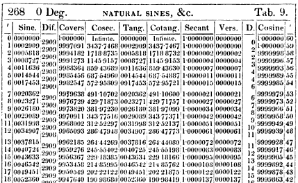
In my previous post the main example of how important mathematical tables were was how astronomical tables were used by mariners to navigate by lunar distance. I don’t actually know the math underlying those astronomical tables so here I’ll use an example I do understand: trigonometric functions. On the right here is a table of trigonometric functions from 1785. It gives 7 digits of the values of 8 different trignonmetric functions, sin, cos, tan, etc., for each arcminute between 0° and 45°. There’s 60 arcminutes to one degree so that’s 2700 values for each function, 21,600 values in total. The author of this table, Charles Hutton, said about this edition in a later one that it had so many errors that is was basically useless:
Finding, as well from the report of others, as from my own experience, that those editions […] were so very incorrectly printed, the errors being multiplied beyond all tolerable bounds, and no dependence to be placed on them for any thing of real practice […]
For this last part about how to calculate complex functions I’ll show how to replicate one column, sin, of this table.
Since we know how to evaluate polynomials the solution that first springs to mind is to approximate the function we want to calculate using a polynomial. Taylor polynomials were well known at this time so that’s an obvious approach. Taylor’s theorem says that for an infinitely differentiable function f (which sin is),
where f(k) means f differentiated n times and a is any point on the function. Since the engine only has 8 columns and we need n+1 columns for a polynomial of degree n we have to limit ourselves to at most the first 7 terms. And in fact, since I want to demonstrate this with the emulator in a little bit and 8 columns of 31 digits takes up an enormous amount of space we’ll limit ourselves even more in this example to 4 columns of 13 digits. This means that we’ll use only the first 3 terms of the Taylor polynomial. For sin those are:
(Conveniently all the even degree terms are 0). This approximates sin quite well around 0 so we’ll use that as the basis for generating the table.
To calculate the differences we first need to produce n+1 values at fixed intervals. The generated table should have an entry per arcminute so we’ll start at 0′ and do steps of 1′:
| x | sin(x) |
|---|---|
| 0’ | 0 |
| 1’ | 2.909 10-4 |
| 2’ | 5.818 10-4 |
| 3’ | 8.727 10-4 |
Then we need to find the nth differences:
| x | sin(x) | Δ1 | Δ2 | Δ3 |
|---|---|---|---|---|
| 0’ | 0 | 2.909 10-4 | -2.461 10-11 | -2.461 10-11 |
| 1’ | 2.909 10-4 | 2.909 10-4 | -4.923 10-11 | |
| 2’ | 5.818 10-4 | 2.909 10-4 | ||
| 3’ | 8.727 10-4 |
All of this is a matter of evaluating a polynomial so that’s not super hard to do by hand with as many decimals as you need, as long as you only need a few of them. From this table we take the last of each of the differences and that’ll be the starting point for the calculation:
0.000872664515235

0.000290888130722

-0.000000000049228

-0.000000000024614
At this point we need to decide how much accuracy we want, that is, where we want the fixed decimal point to be. We have 13 digits which gives us room enough to multiply by 1013 before rounding. That gives us these integer values:
8726645152

2908881307

-492

-246
And now we’re ready to get tabulating:

If you follow along with the original table you can see that it generates exactly the same values. The values generated by the engine continue to match the table values until 1° 1′, 57 values in, where the table says 0.0177432 and the engine produces 0.0177433, and after that it continues to produce matching values up until 1° 53′, more than 100 values in.
Not bad right? And remember, this is a simplified emulator that can only calculate the third degree approximation where the original could go up to the seventh, and only with 13 digits of precision where the original had 31.
So what’s the source of the deviation? There’s two: the approximating polynomial and the accumulating error of the engine. Let’s first look at the polynomials.

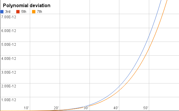
This is a plot of how quickly the approximating polynomials of different degrees deviate from the true sine function. At 1° the approximations are still well within 0.01 billionth of the correct value. Like I said, near 0 these polynomials approximate sin really well.
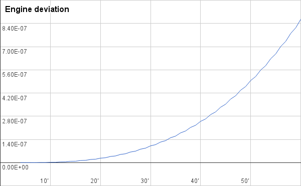
This suggests that the main source of inaccuracy is the engine itself, the precision we had to discard when fixing the decimal point, and as you can see in the second graph, it is. The engine loses precision faster than the polynomial by a large factor. This makes sense because the inaccuracy accumulates for every step.

Luckily in this case the polynomial deviates slowly enough we can use it to calculate new almost-accurate initial values at fixed intervals, for instance for each degree, and reset the machine to those. However, eventually the polynomial itself will deviate too much and at that point we can use the fact that the Taylor polynomial has an a parameter that specifies the point around which we’re approximating. So say the polynomial that approximates around 0° becomes too inaccurate at 6° we can derive a Taylor polynomial around 6° and use that to continue the calculation. Indeed, since the polynomial approximates equally well on both sides of the point we might as well approximate around 9° and use it for all values between 6° and 12°.
Sin is a relatively easy function to approximate in this way, a function such as log is harder but the same basic principles apply to harder functions. It’s a matter of how often you need to reset to get rid of the accumulating errors and how long the same approximating polynomial remains accurate.
One of the weak points of the engine is that even though it requires less manual work than producing a table completely manually, there’s still a fair amount of manual analysis and computation to be done. That’s not a killer in itself though. Even if it took just as much work to operate, which it surely wouldn’t have, just having a different way to create these tables would have been immensely valuable since two different approaches are likely to produce different errors and hence can be used to cross-check each other. But as this illustrates, even if the engine had been built it was definitely not a matter of just plugging in a few values and then going to lunch, using it involved a fair amount of work4.
The revolution that didn’t happen
Here’s a video of the only difference engine ever built which was completed in 2002.
Babbage tried to build it and ultimately gave up for a number of reasons including family problems, financial problems, problems working with his engineer, and his gradual change of focus to the analytical engine. Despite what you often hear the technology did exist to build it; the modern one was built from his designs and only with technology that would have been available back then.
It also appears that Babbage’s interests and those of the English government who paid for the whole thing were just too far apart. Babbage was interested in the machine itself whereas his sponsors just wanted accurate tables, whatever way Babbage could produce them. It’s a shame really. It seems from what I’ve read that the difference engine was a failure not of vision or technology but of product management. The technology was so promising that if a successful prototype had been built and he’d delivered the tables the English government wanted it’s not unlikely that they would have continued to fund research in more advanced engines. The ground would have been fertile for mechanical calculation on a larger scale by the mid 1800s. Obviously that wouldn’t have meant a mechanical iPad in every home by 1900 but it would certainly have been a better outcome than what happened, that the designs went in the drawer.
Ultimately Babbage moved on to the analytical engine, the first ever programmable computer. My next post will be about that and in particular the first ever software programs which were written for it.
Sources
For more information about the difference engine a quick introduction is given in the first part of Menabrea’s Sketch of the Analytical Engine from 1842. A more detailed description, including of the underlying mechanics of the engine, can be found in Lardner’s Babbage’s Calculating Engine from the July 1834 edition of the Edinburgh Review.
Notes
-
While the emulator performs the same type of calculations as the difference engine it actually looks nothing like it. I made a point to give the emulator a mechanical feel but it’s inspired more by the Curta calculator, the mechanical calculator I know best, not the difference engine. Note also that I have only tested it on the browsers I have easy access to, Chrome, Firefox, Opera, and Safari on mac. If it doesn’t work on your platform the code lives on github and patches are welcome. ↩
-
Ada Lovelace in her famous notes about it is almost contemptuous of how simple it is compared to the analytical engine:
The Difference Engine can in reality […] do nothing but add; and any other process […] can be performed by it only just to the extent in which it is possibly, by judicious mathematical arrangement and artifices, to reduce them to a series of additions.
-
Incidentally, much of the underlying math was developed before Babbage by J. H. Müller. ↩
-
I wonder if it’s possible to automate some of the manual work involved in operating the engine using the engine itself, like calculating initial values. ↩